Optimization
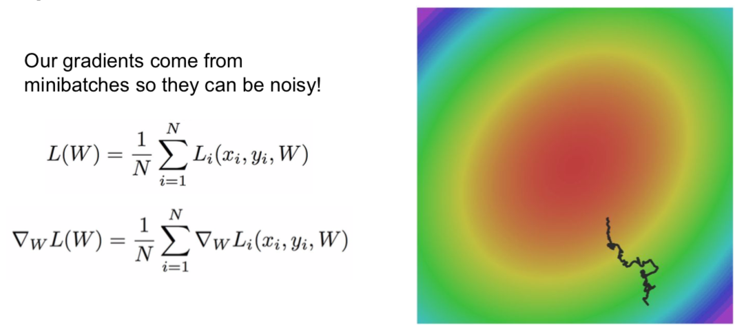
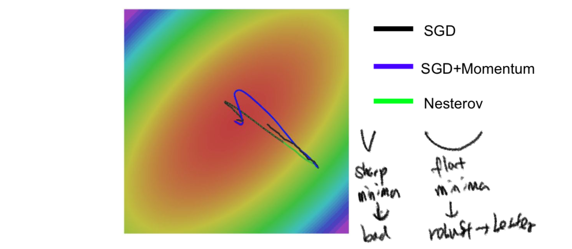
- problem with SGD

- the slope is small horizontally and steep vertically
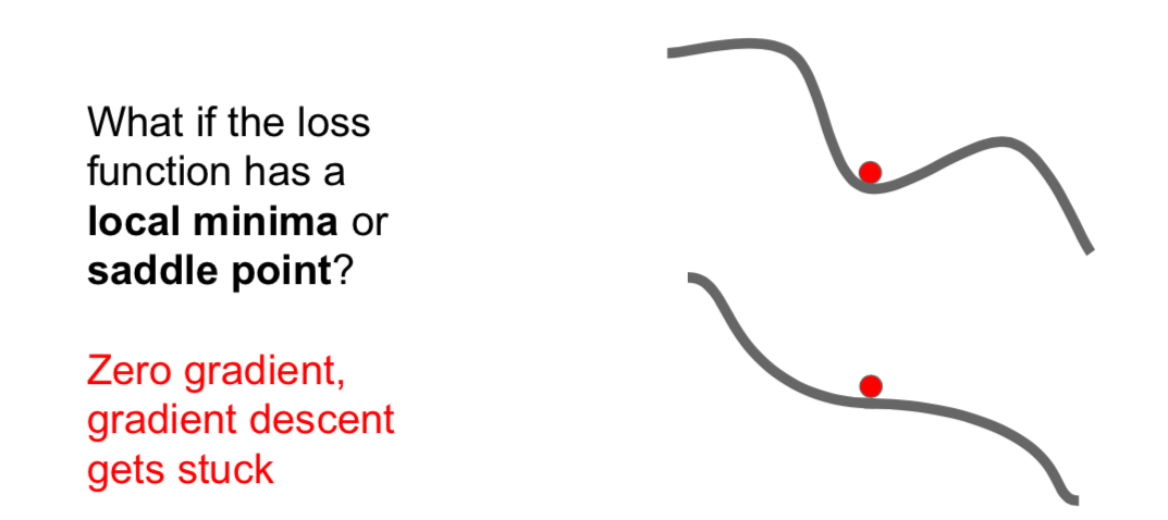
- in practice, saddle points occur more frequently in higher dimensions
- saddle point: it is a point that is maximum on one axis in a multivariate function, but minimum on some axes.
- SGD + Momentum
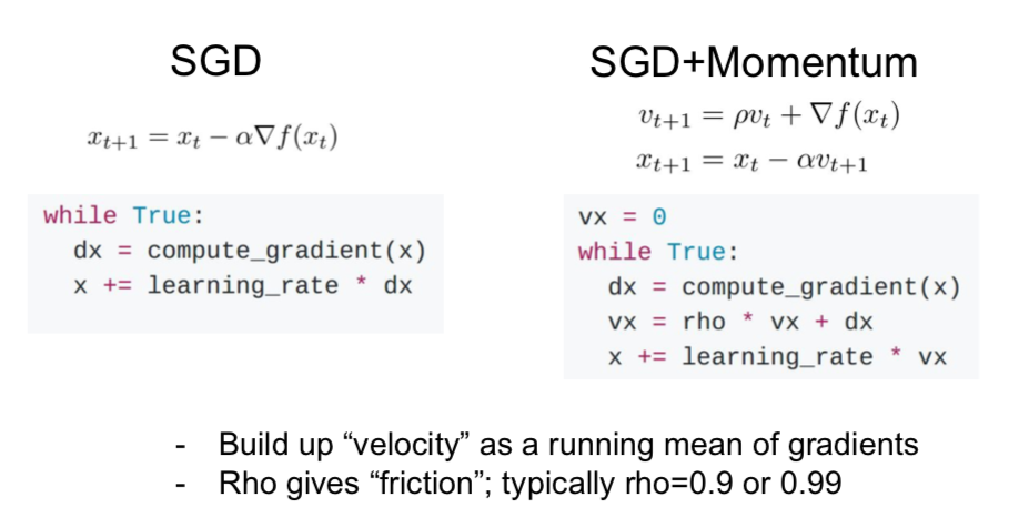
- because acceleration is considered, it continues even when the speed reaches zero
- \(\rho\): hyperparameter to slow down

- Nesterov Momentums
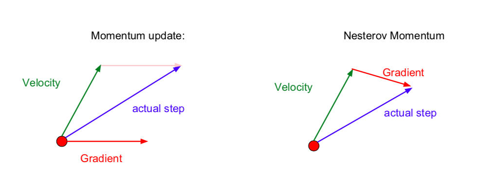
- SGD + Momentum: Velocity + Gradient -> acutal step
- Nesterov: Velocity -> Gradient -> actual step (after moving towards velocity, calculate the acutal step by obtaining gradients)
- \(v_{t+1} = \rho v_t - \alpha \triangledown f(x_t + \rho v_t)\) (reflect the latest speed as a greater weight)
- \[x_{t+1} = x_t + v_{t+1}\]
- \(v_t\) initialization = 0
- \(x_t + \rho v_t\): move towards velocity and get the gradient
- \(when \ \tilde x_t = x_t + \rho v_t\), (to make loss function suitable for use)
- \[v_{t+1} = \rho v_t - \alpha \triangledown f(\tilde x_t)\]
- \[\tilde x_{t+1} = \tilde x_t - \rho v_t + (1 + \rho) v_{t+1} = \tilde x_t + v_{t+1} + \rho(v_{t+1} - v_t)\]
- AdaGrad

- Q. What happens with AdaGrad?
- Slow-moving dimensions move fast, fast-moving dimensions move slowly, because dividing by squared gradients makes the rate of updates constant in all dimensions
- Q. What happensto the step size over long time?
- because squared gradients are added, step size is reduced
- In practice, it’s rarely used.
- RMSProp
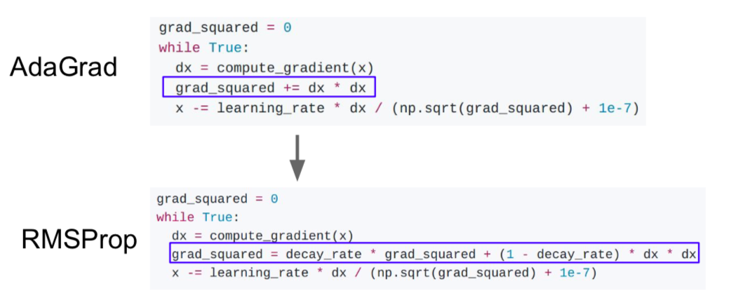
- The decay rate prevents the squared gradients from growing rapidly
- Decay rate is usually 0.9 or 0.99
- Adam
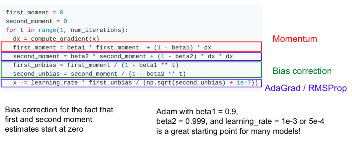
- a combination of Momentum and RMSPro.
- Q. What happens at first timestep when unbiases are missing?
- Because ‘second_moment’ is close to zero, x will be a very small number. So at first it moves in a very big step. In some cases, however, this doesn’t occur because the ‘first_moment’ is also offset by being close to zero.
- In most cases, use Adam.
- Learning rate in optimizer

- it was suggested in ‘Resnet’ that the loss is reduced by reducing the learning rate while circling the epoch
- First-Order Optimization
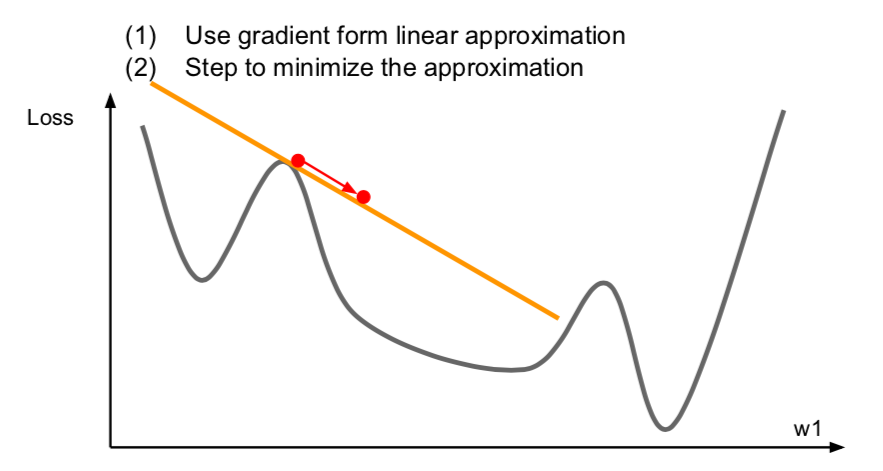
- this concept used so far, calculating gradients at a point.
- Second-Order Optimization
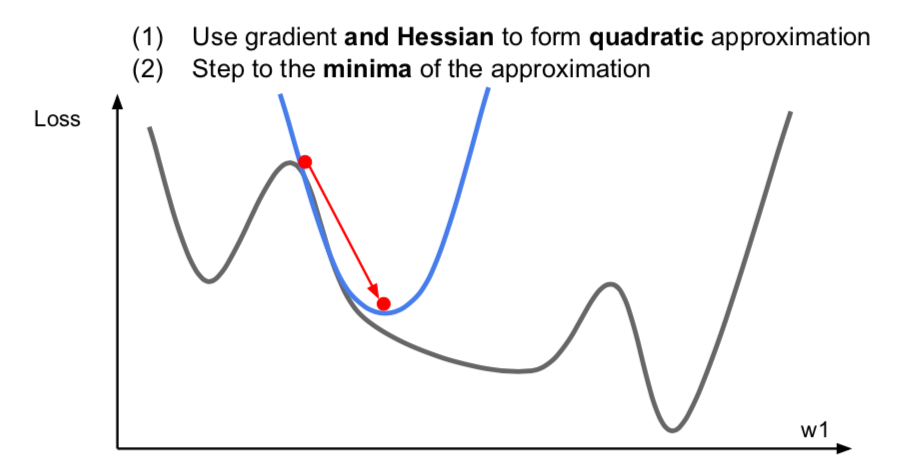
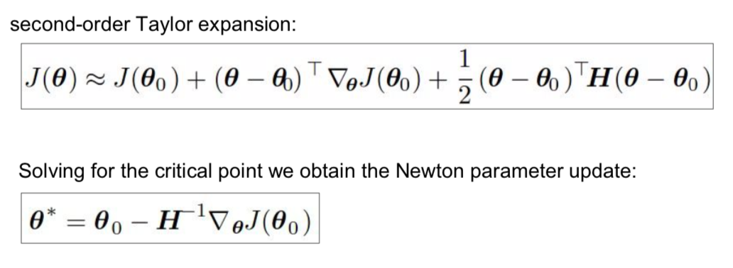
- it uses a quadratic approximation to find the value.
- Q. What is nice about this update?
- No hyperparameters, No learning rate
- Q. why is this bad for deep learning?
- Hessian has \(O(N^2)\) elemetns. Inverting takes \(O(N^3)\). N = (Tens or Hundreds of) Millions
- if the matrix becomes larger, it cannot be stored in memory
- Optimization
- BGFS
- instead of inverting the Hessian (\(O(n^3)\)), approximate inverse Hessian with rank 1 updates over time (\(O(n^2)\) each)
- L-BFGS
- doesn’t form/store the full inverse Hessian
- usually works very well in full batch, deterministic mode
- does not transfer very well to mini-batch setting
- doesn’t work well in deep learning (stochastic problem, non-convex problem, etc)
- BGFS
- Model Ensembles
- train multiple independent models and average their results at test time \(\rightarrow\) 2% extra performance
- instead of training independent models, use multiple snapshots of a single model
- instead of using actual parameter vector, keep a moving average
- using a smoothly decaying average
- not too common in practice
Regularization
- ways to improve single-model performance
- Adding term to loss

- add a regulation on the loss function
- it is not commonly used in deep learning
- Dropout
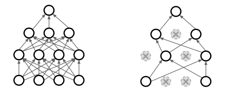
- deactivate random neurons when passing through neural networks
- common to deactivate values below 0.5
- Q. How can this possibly be a good idea?

- prevents co-adaptation of features \(\rightarrow\) prevents overfitting

- a large ensemble of models that share parameters
- an ensemble effect because each neuron has different subsets
- test time
- “average out” the randomness at test-time

- output at the test-time = probability * output at training time
- Inverted Dropout
- Batch Normalization
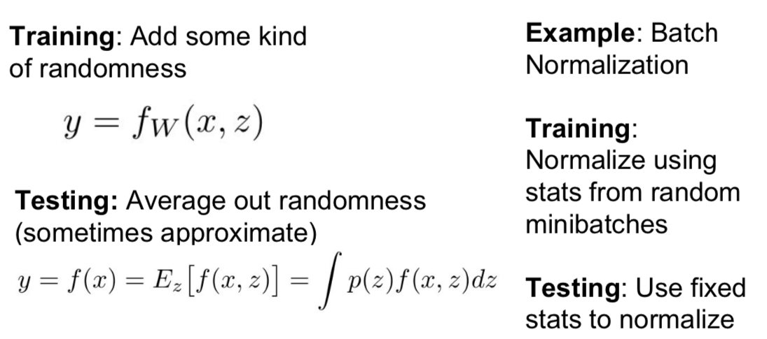
- normalize each minibatch randomly during training
- during testing, the same normalization is performed on all data
- Data Augmentation
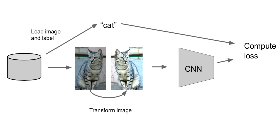
- make various images by modifying images
- by combining various images, there is a regulatory effect to prevent overfitting
- horizontal flips, random crops and scales, color jitter, color offset, etc
- DropConnect

- activation을 0으로 만드는 것이 아니라 임의의 weight matrix 값을 0으로 한다.
- Fractional Max Pooling
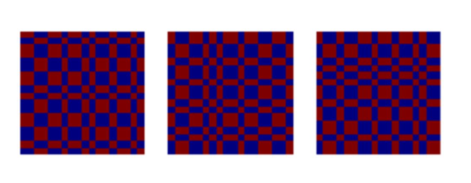
- select random area when pooling
- at the test time, freeze the pooling region or average out of several pooling regions
- not commonly used
- Stochastic Depth

- drop some layers during training
- all layers are used for test time
- similar effect to dropout

Transfer Learning
- Using a pre-trained model.
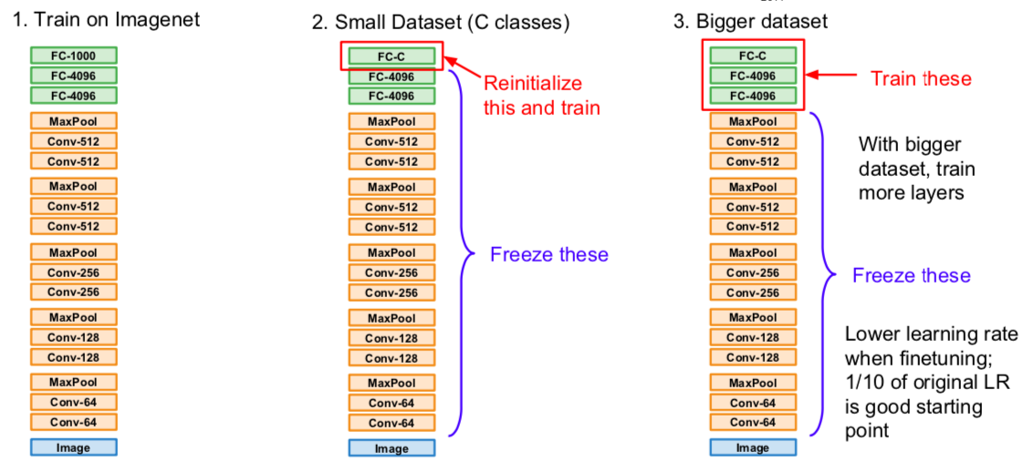
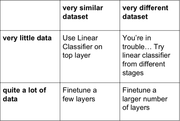
- small dataset: transform only the last layer of the pre-trained model, freeze the other layers, and train
- bigger dataset: train by transforming more layers than in the above way. Because the pre-trained model is well trained, set the learning rate small
- When using CNN, transfer learning is usually used, rather than training everything from the beginning.
This is written by me after taking CS231n Spring 2017 provided by Stanford University.
If you have questions, you can leave a reply on this post.