Supervised vs Unsupervised Learning
- Supervised Learning
- Data: (x, y) \(\rightarrow\) x: data, y: label
- Goal: learn a function to map x \(\rightarrow\) y
- Examples: classification, regression, object detection, semantic segmentation, image captioning, etc
- Unsupervised Learning
- Data: data without label (training data is cheap)
- Goal: learn some underlying hidden structure of the data
- Examples: clustering, dimensionality reduction, feature learning, density estimation, etc
Generative Models
- Given training data, generate new samples from same distribution
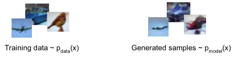
- Want to learn \(p_{model}(x)\) similar to \(p_{data}(x)\)
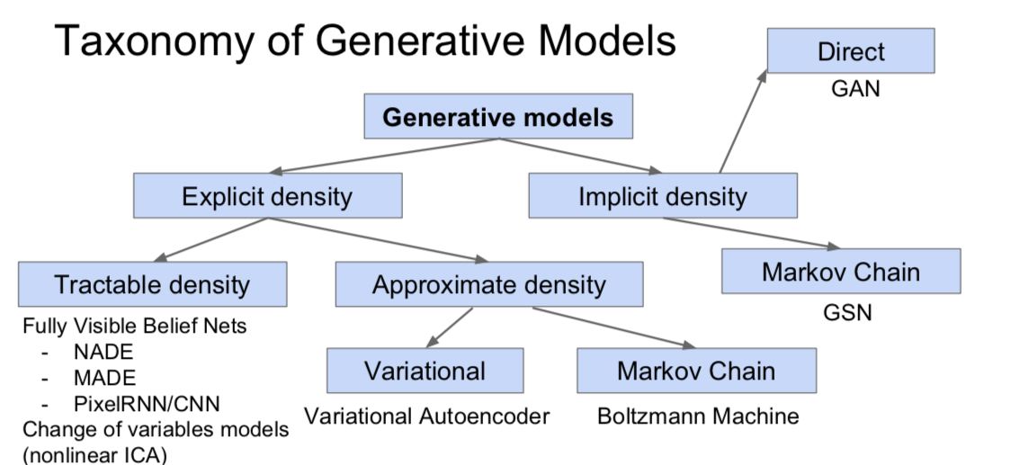
- Ways
- Explicit density estimation: explicitly define and solve for \(p_{model}(x)\)
- Implicit density estimation: learn model that can sample from \(p_{model}(x)\) w/o explicitly defining it
- Why Generative Models?
- Realistic samples for artwork, super-resolution, colorization, etc
- Generative models of time-series data can be used for simulation and planning (reinforcement learning applications!)
- Training generative models can also enable inference of latent representations that can be useful as general features (latent = hidden)
PixelRNN and PixelCNN
- Explicit density model
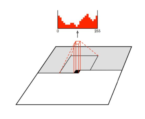
- Use chain rule to decompose likelihood of an image x into product of 1-d distributions by a neural network (explicitly compute)
- \(p(x) = \prod^n_{i=1} p(x_i \vert x_1, \cdots, x_{i-1})\) (\(p(x)\): likelihood of image x, \(x_i\): probability of i’th pixel value given all previous pixels)
- maximize likelihood of training data
- explicit likelihood of training data gives good evaluation metric
- PixelRNN
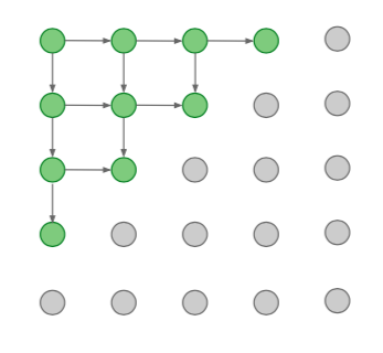
- Generate image pixels starting from corner
- Dependency on previous pixels modeled using an RNN (LSTM)
- Drawback: sequential generation is very slow
- PixelCNN
- Generate image pixels starting from corner
- Dependency on previous pixels modeled using a CNN over context region
- Training: maximize likelihood of training images \(p(x)\)
- Faster than PixelRNN, but still slow because it proceeds sequentially
Variational Autoencoders (VAE)
- \[p_{\theta}(x) = \int p_{\theta}(z)p_{\theta}(x \vert z)dz\]
- Cannot optimize directly, derive and optimize lower bound on likelihood instead
- Background: Autoencder
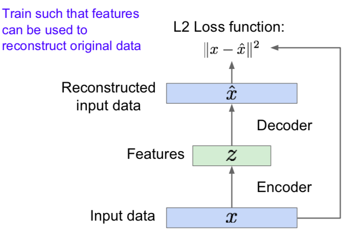
- Unsupervised approach for learning a lower-dimensional feature representation from unlabeled training data
- Encoder
- Originally: Linear + nonlinearity (sigmoid)
- Later: Deep, fully-connected
- Later: ReLU CNN
- z usually smaller than x (dimensionality reduction, capture meaningful factors)
- Decoder
- Originally: Linear + nonlinearity (sigmoid)
- Later: Deep, fully-connected
- Later: ReLU CNN (upconv)
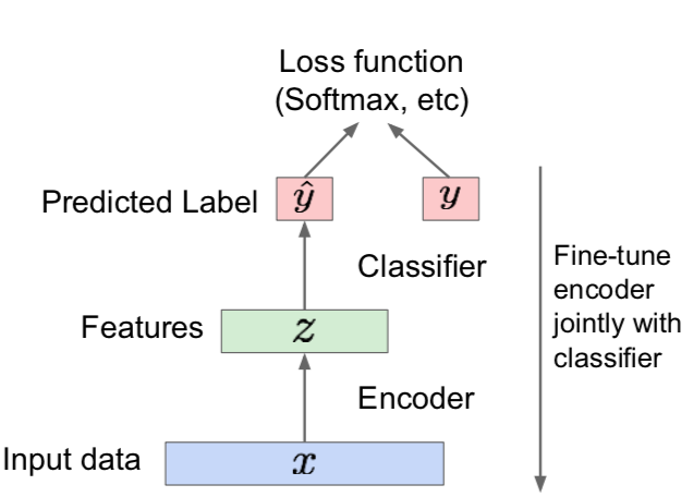
- After training, throw away decoder
- Encoder can be used to initialize a supervised model
- Variational Autoencoders
- sample from the model to generate data
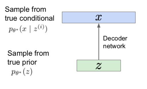
- How to represent the model
- Choose prior p(z) to be simple, e.g. Gaussian
- Conditional p(x \vert z) is complex (generates image), so represent with neural network
- How to train the model
- Learn model parameters to maximize likelihood of training data, but it is intractable
- Data likelihood: \(p_{\theta}(x) = \int p_{\theta}(z)p_{\theta}(x \vert z)dz\)
- \(p_{\theta}(z)\): by simple Gaussian prior
- \(p_{\theta}(x \vert z)\): Decoder neural network
- \(\int\): Intractible to compute \(p(x \vert z)\) for every z
- Posterior density: \(p_{\theta}(z \vert x) = p_{\theta}(x \vert z)p_{\theta}(z)/p_{\theta}(x) \rightarrow p_{\theta}(x)\): Intractable
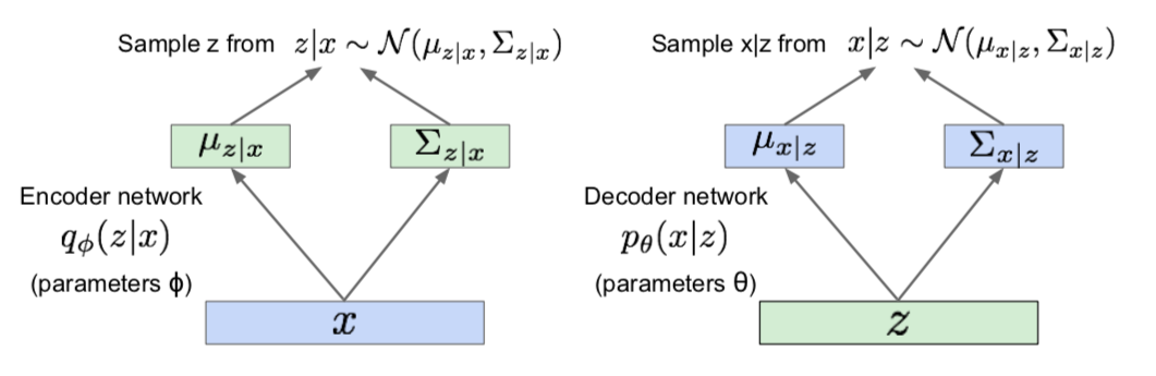
- Solution: In addition to decoder network modeling \(p_{\theta}(x \vert z)\), define additional encoder network \(q_{\phi}(z \vert x)\) that approximates \(p_{\theta}(z \vert x)\)
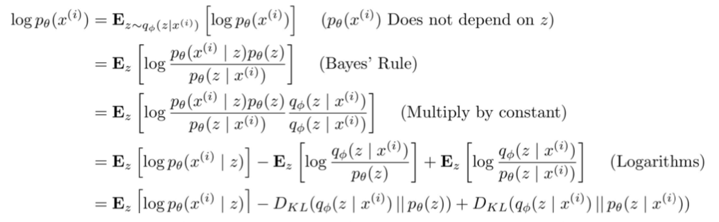
- \(E_z[ log p_{\theta} (x^{(i)} \vert z ]\): compute estimate through sampling
- \(D_{KL}(q_{\phi}(z \vert x^{(i)}) \vert \vert p_{\theta}(z))\): has closed-form solution
- \(D_{KL}(q_{\phi}(z \vert x^{(i)}) \vert \vert p_{\theta}(z \vert x^{(i)}))\): intractable \(\rightarrow p_{\theta}(z \vert x^{(i)})\), but KL divergence always \(\geq 0\)
- Think of the first two calculable terms (\(L(x^{(i)}, \theta, \phi)\)) as the lower bound and maximize them
Generative Adversarial Networks (GAN)
- GAN: don’t work with any explicit density function, instead learn to generate from training distribution through 2-player game
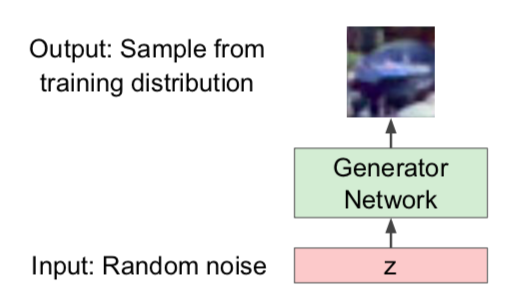
- Sample from a simple distribution
- Learn transformation to training distribution
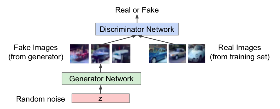
- Generator network: try to fool the discriminator by generating real-looking images
- Discriminator network: try to distinguish between real and fake images
- Trainig GAN
- Gradient descent on generator
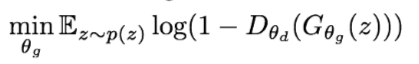
- to minimize objective such that D(G(z)) is close to 1 (discriminator is fooled into thinking generated G(z) is real)
- Gradient ascent on discriminator
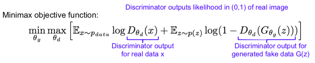
- to maximize objective such that D(x) is close to 1 (real) and D(G(z)) is close to 0 (fake)
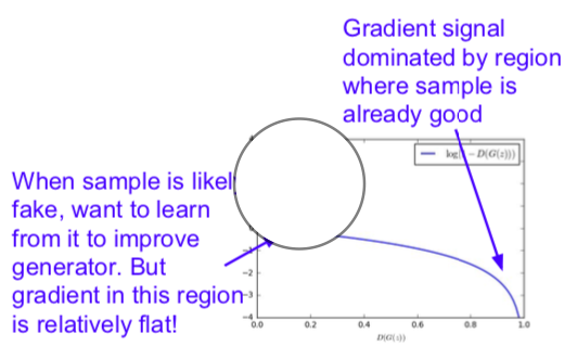
- In practice, optimizing this generator objective does not work well
- When D(G(z) is small, training should be allowed to proceed, but learning does not work well because of small gradient, and when D(G(z) is large, training is not necessary, but training proceeds because of big gradient
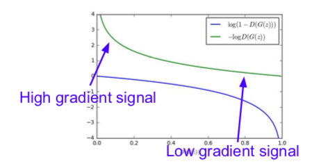
- Maximize likelihood of discriminator being wrong
- Same objective of fooling discriminator, but now higher gradient signal for bad samples => works much better! (standard in practice)
- Aside: Jointly training two networks is challenging, can be unstable. Choosing objectives with better loss landscapes helps training (active area of research)
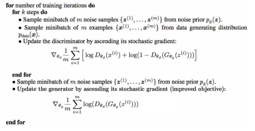
- Gradient descent on generator
- GAN: Convolutional Architectures
- It is said that applying the CNN architecture to GAN improves performance quite a bit
- Generator: an upsampling network with fractionally-strided convolutions
- Discriminator: convolutional network

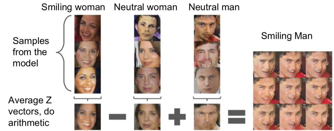
- GAN: Interpretable Vector Math
This is written by me after taking CS231n Spring 2017 provided by Stanford University.
If you have questions, you can leave a reply on this post.