What is Reinforcement Learning?
- Problems involving an agent interacting with an environment, which provides numeric reward signals (objective, state, action, reward)
- Goal: Learn how to take actions in order to maximize reward
- Keep going until the environment gives back a termianl state
- Example: Cart-Pole problem, Robot Locomotion, Atari Games, Go
Markov Decision Processes
- Mathematical formulation of the RL problem
- Markov property: No matter what time a specific state is reached or what state has been gone through before, the probability of going to the next state is always the same
- Symbols
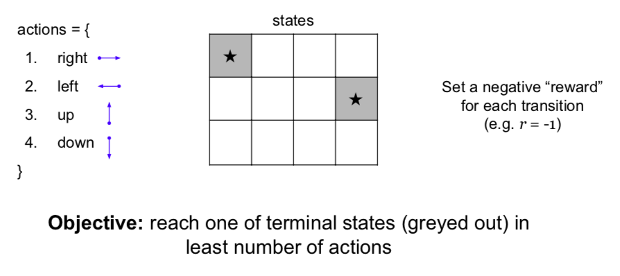
- S: set of possible states
- A: set of possible actions
- R: distribution of reward given (state, action) pair
- P : transition probability i.e. distribution over next state given (state, action) pair
- \(\gamma\): discount factor
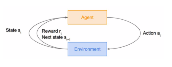
- Steps
- At time step t=0, environment samples initial state \(s_0 \rightarrow p(s_0)\)
- Then, for t=0 until done:
- Agent selects action \(a_t\)
- Environment samples reward \(r_t \rightarrow R( . \vert s_t, a_t)\)
- Environment samples next state \(s_{t+1} \rightarrow P( . \vert s_t, a_t)\)
- Agent receives reward \(r_t\) and next state \(s_{t+1}\)
- A policy \(\pi\): function from S to A that specifies what action to take in each state
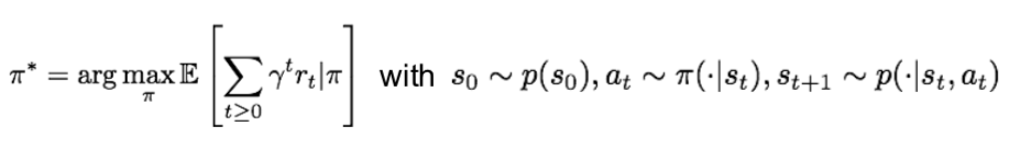
- Objective: find policy \(\pi^*\) that maximizes cumulative discounted reward: \(\sum_{t \geq 0} \gamma^t r_t\)
- Example: Grid World
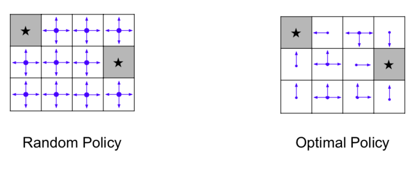
- Optimal Policy is more efficient than Random Policy
- Optimal Policy \(\pi^*\)
- Maximizes the sum of rewards
- handle the randomness (initial state, transition probability…) \(\rightarrow\) Maximize the expected sum of rewards
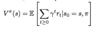
- Value Function
- at state s, the expected cumulative reward from following the policy from state s
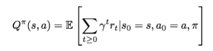
- Q-value function
- at state s and action a, the expected cumulative reward from taking action a in state s and then following the policy
- Bellman Equation
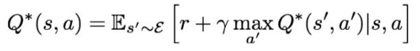
- the sum of the reward at that point and the expected reward afterwards
- if the optimal state-action values for the next time-step Q are known, then the optimal strategy is to take the action that maximizes the expected value
- use Bellman equation as an iterative update
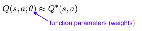
- Problem: not scalable. Must compute Q(s,a) for every state-action pair. If state is e.g. current game state pixels, computationally infeasible to compute for entire state space
- Solution: use a function approximator to estimate Q(s,a). E.g. a neural network!
Q-Learning
- Q-Learning
- Use a function approximator to estimate the action-value function
- Deep q-learning: when the function approximator is a deep neural network
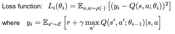
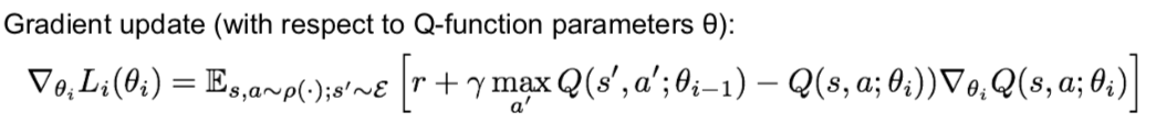
- Forward Pass
- Backward Pass
- Q-network Architecture
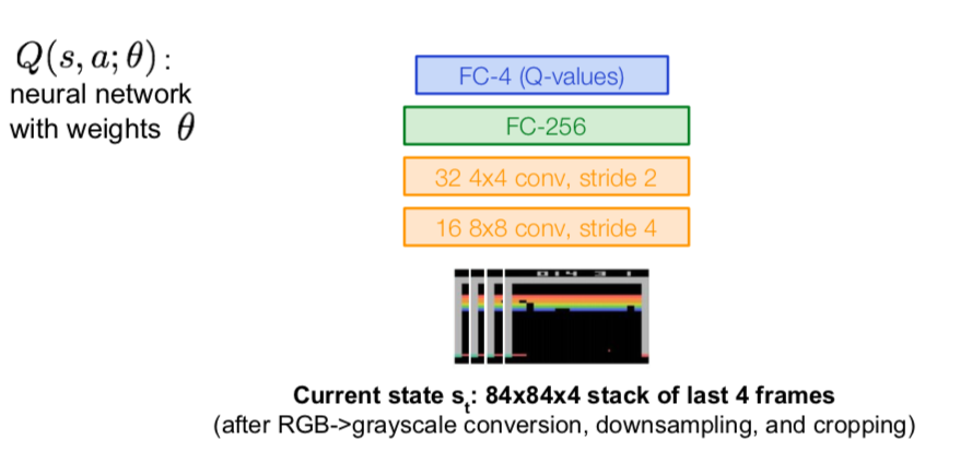
- Input: state \(s_t\)
- Output: 4-d output (if 4 actions), corresponding to \(Q(s_t, a-1), Q(s_t, a_2), Q(s_t, a_3), Q(s_t, a_4)\)
- Advantage: a single feedforward pass to compute Q-values for all actions from the current state \(\rightarrow\) efficient
- Experience Replay
- Learning from batches of consecutive samples is problematic
- samples are correlated \(\rightarrow\) inefficient learning
- current Q-network parameters determines next training samples \(\rightarrow\) lead to bad feedback loops
- Solution: Experience Replay
- continually update a replay memory table of transitions \((s_t, a_t, r_t, s_{t+1})\) as game (experience) episodes are played
- train Q-network on random minibatches of transitions from the replay memory, instead of consecutive samples
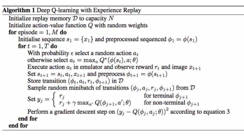
- initialize replay memory, Q-network
- play M episodes (full games)
- initialize state (starting game screen pixels) at the beginning of each episode
- with small probability, select a random action (explore), otherwise select greedy action from current policy
- take the action \((a_t)\), and observe the reward \(r_t\) and next state \(s_{t+1}\)
- store transition in replay memory
- Experience Replay: sample a random minibatch of transitions from replay memory and perform a gradient descent step
- Learning from batches of consecutive samples is problematic
Policy Gradients
- What is a problem with Q-learning? \(\rightarrow\) The Q-function can be very complicated!
- very high-dimensional state \(\rightarrow\) hard to learn exact value of every (state, action) pair
- Policy Gradients
- parametrized policies: \(\Pi = {\pi_{\theta}, \theta \in R^m}\)
- value: \(J(\theta) = E[\sum_{t \geq 0} \gamma^t r_t \vert \pi_{\theta}]\)
- optimal policy: \(\theta^* = arg max_{\theta} J(\theta) \rightarrow\) Gradient ascent
- Reinforce Algorithm
- Expected reward: \(J(\theta) = E_{\tau \sim p(\tau ; \theta)[ r(\tau) ]} = \int_{\tau} r(\tau)p(\tau ; \theta) d \tau\)
- (\(\tau = (s_0, a_0, r_0, s_1, \cdots)\): reward of a trajectory)
- cf)
- \(\triangledown_{\theta} J(\theta) = \int_\tau r(\tau) \triangledown_{\theta} p(\tau ; \theta) d \tau \rightarrow\) intractable when gradient of an expectation is problematic when p depends on θ
- \[\triangledown_{\theta} J(\theta) = p(\tau ; \theta) {\triangledown_{\theta} p(\tau ; \theta) \over p(\tau ; \theta)} = p(\tau ; \theta) \triangledown_{\theta} log \ p(\tau ; \theta)\]
- \(\triangledown_{\theta} J(\theta) = \int_\tau (r(\tau) \triangledown_{\theta} log \ p(\tau ; \theta)) p(\tau ; \theta)d \tau \rightarrow\) estimate with Monte Carlo sampling
- without knowing the transition probabilities
- \[p(\tau ; \theta) = \Pi_{t \geq 0} p(s_{t+1} \vert s_t, a_t) \pi_{\theta} (a_t \vert s_t)\]
- \[log \ p(\tau ; \theta) = \sum_{t \geq 0} log \ p(s_{t+1} \vert s_t, a_t) + log \ \pi_{\theta} (a_t \vert s_t)\]
- \(\triangledown_{\theta} log \ p(\tau ; \theta) = \sum_{t \geq 0} \triangledown_{\theta} log \ \pi_{\theta} (a_t \vert s_t) \rightarrow\) doesn’t depend on transition probabilities
- \(\triangledown_{\theta} J(\theta) \approx \sum_{t \geq 0} r(\tau) \triangledown_{\theta} log \ \pi_{\theta} (a_t \vert s_t) \rightarrow\) can estimate \(J(\theta)\)
- if \(r(\tau)\)(= reward) is high, push up the probabilities of the actions seen
- if \(r(\tau)\) is low, push down the probabilities of the actions seen
- however, since the value is averaged out while calculating all values as an expected value, it is difficult to know exactly what action is good, that is, the variance value for the reward of the best action is too large
- variance reduction
- first idea: instead of considering the overall reward, the best choice is made by considering only the reward from the current state to the end
- second idea: use discount factor \(\gamma\) to ignore delayed effects, in other words, it means distinguishing between rewards to be received immediately and rewards to be received in the distant future
- Baseline
- The raw value of a trajectory isn’t necessarily meaningful, but Whether a reward is better or worse than what to be expected to get
- \[\triangledown_{\theta} J(\theta) \approx \sum_{t \geq 0} (\sum_{t^` \geq t} \gamma^{t`-t} r_{t^`} - b(s_t)) \triangledown_{\theta} log \Pi_{\theta} (a_t \vert s_t)\]
- \(b(s_t)\): constant moving average of rewards experienced so far from all trajectories
- find out if the current reward was good or bad compared to the previous one
- there are used in “Vanilla Reinforce”
- Better Baseline
- by using Q-function and value function
- happy with large \((Q^{\Pi_{\theta}} (s_t, a_t) - V^{\Pi_{\theta}} (s_t))\)
- \[\triangledown_{\theta} J(\theta) \approx \sum_{t \geq 0} (Q^{\Pi_{\theta}} (s_t, a_t) - V^{\Pi_{\theta}} (s_t)) \triangledown_{\theta} log \Pi_{\theta} (a_t \vert s_t)\]
- Actor-Critic Algorithm
- problem: don’t know Q and V
- solution: using Q-learning \(\rightarrow\) combine Policy Gradients and Q-learning by training both an actor (the policy) and a critic (the Q-function)
- actor: decide which action to take
- critic: tell the actor how good its action was and how it should adjust
- alleviates the task of the critic as it only has to learn the values of (state, action) pairs generated by the policy
- incorporate Q-learning tricks (e.g. experience replay)
- advantage function: how much an action was better than expected
- \[A^{\pi}(s,a) = Q^{\pi}(s,a) - V^{\pi}(s)\]

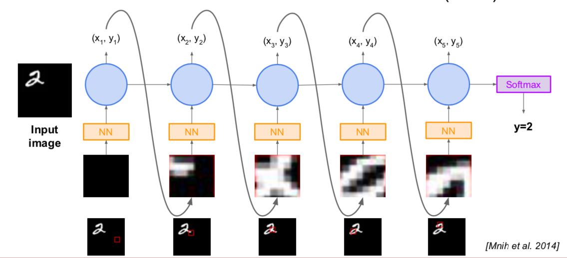
- Recurrent Attention Model (RAM)
- objective: Image Classification
- take a sequence of “glimpses” selectively focusing on regions of the image, to predict class
- inspiration from human perception and eye movements
- saves computational resources \(\rightarrow\) scalability
- able to ignore clutter / irrelevant parts of image
- glimpsing is a non-differentiable operation \(\rightarrow\) learn policy for how to take glimpse actions using REINFORCE
- state: glimpses seen so far
- action: (x,y) coordinates (center of glimpse) of where to look next in image
- reward: 1 at the final timestep if image correctly classified, 0 otherwise
This is written by me after taking CS231n Spring 2017 provided by Stanford University.
If you have questions, you can leave a reply on this post.