Activation Functions
- Sigmoid
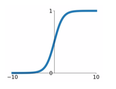
- \[\sigma (x) = 1/(1+e^{-x})\]
- squashes numbers to range [0,1]
- historically popular
- problems
- saturated nuerons kill the gradients (saturate: converging to a constant value)
- at some point, the gradient becomes zero.
- outputs are not zero-centered
- since input is always positive, gradients on w are always all positive or negative
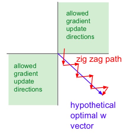
- since input is always positive, gradients on w are always all positive or negative
- exp() is a bit compute expensive
- it’s less complicated than convolution and dot product, but it can still be a problem
- saturated nuerons kill the gradients (saturate: converging to a constant value)
- tanh(x)
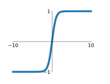
- squashes numbers to range [-1,1]
- zero centered
- kills gradients when saturated
- better than sigmoid
- ReLU (Rectified Linear Unit)
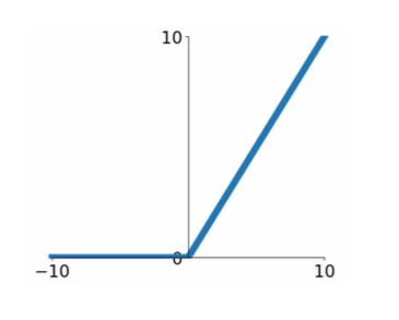
- \[f(x) = max(0,x)\]
- does not saturate (in + region)
- computationally efficient
- convergence is much faster than sigmoid/tanh in practice
- more biologically plausible than sigmoid
- issues
- not zero-centered output
- saturatation when \(x \leq 0\)
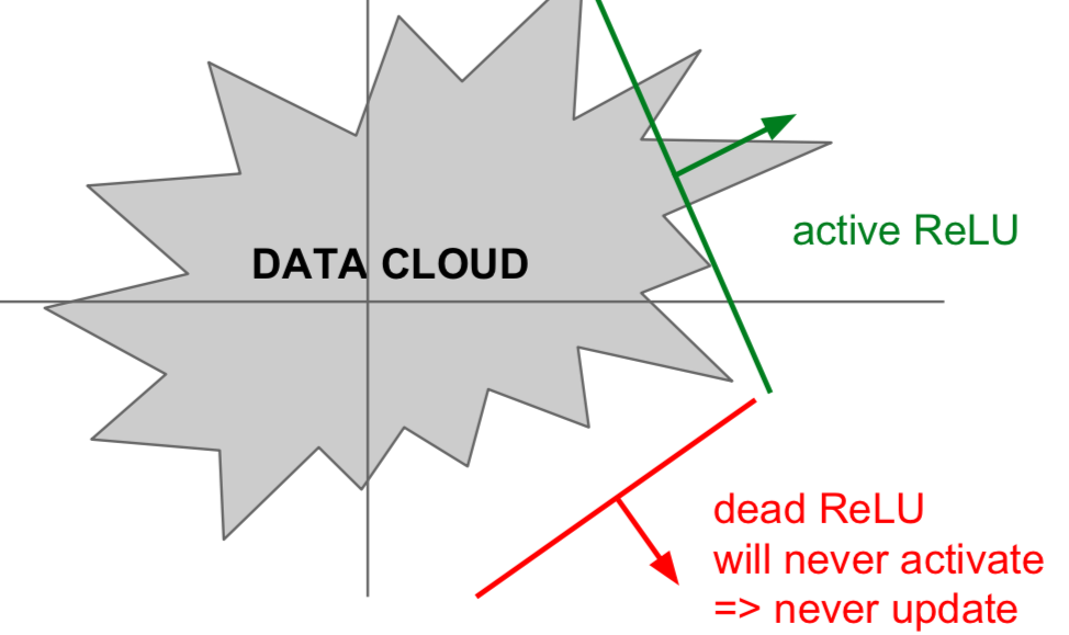
- dead ReLU occurs when there is an error in the initial value setting or the learning rate is too large. If the learning rate is too large and w becomes equal to or less than zero, then it becomes a dead ReLU from that point on.
- Leaky ReLU
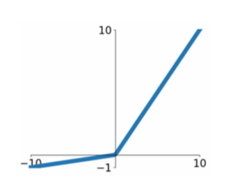
- \[f(X) = max(0.01x, x)\]
- does not saturate
- computationally efficient
- converges much faster than sigmoid/tanh in practice
- will not die
- PReLU (Parametric Rectifier)
- \[f(x) = max(\alpha x, x)\]
- \(\alpha\): parameter, determined by backprops
- more flexible
- ELU (Expoential Linear Units)
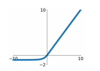
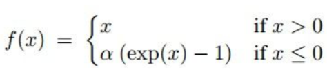
- all benefits of ReLU
- closer to zero mean outputs
- negative saturation regime compared with Leaky ReLU adds some robustness to noise
- compuatation requires exp()
- Maxout Neuron
- \[max(w_1^Tx + b_1, w_2^Tx + b_2)\]
- does not have the basic form of dot product -> nonlinearity
- generalizes ReLU and Leaky ReLU
- Linear segime, No saturation, Never die
- doubles the number of parameters/neuron
- Conclusion: “Use ReLU!”
Data Preprocessing
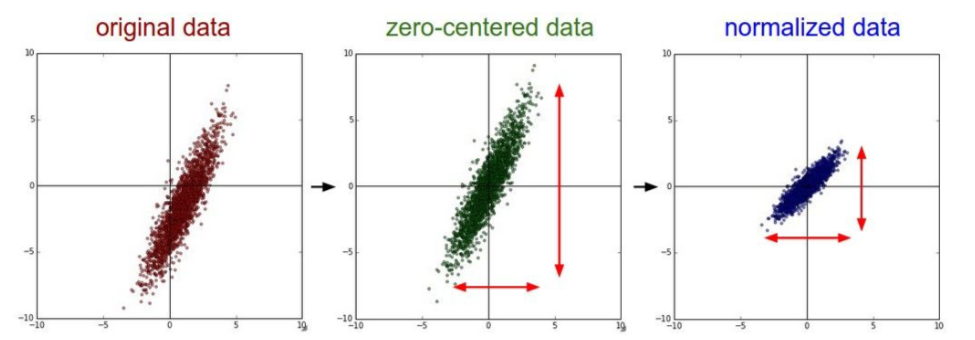
- Zero-centering
- subtract the mean image (e.g. AlexNet)
- subtraact per-channel mean (e.g. VGGNet)
- Normalization: the image is not in this process because it is already somewhat normalized.
- PCA/Whitening: images do not perform this process because spatial characteristics are used.
Weight Initialization
- W = 0
- all neurons do the same operation (occurs if all ‘w’s are same)
- Small random numbers
-
W = 0.01 * np.random.randn(D, H) # generating Gaussian normal distribution random numbers with mean 0, standard deviation 1 in D X H matrix - Works well for small networks, but problems with deeper networks
- using tanh as an activation function,
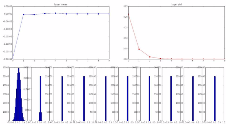
- smaller slopes gradually disappear and only around zero remains
- the gradient is zeroed at backpropagation
- using tanh as an activation function,
-
- Bigger random numbers
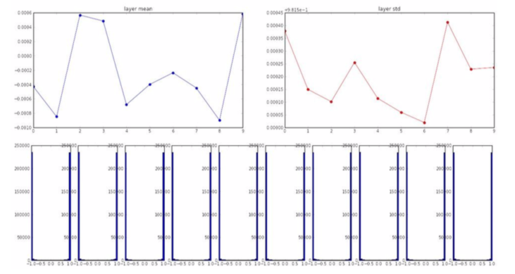
- almost all neurons completely saturated, either -1 and 1. Gradients will be all zero. No updating!
- Xavier initialization
- divide by the number of inputs
-
W = np.random.randn(fan_in, fan_out) / np.sqrt(fan_in) - when using nonlinearity, it kills the half of units -> bad
- improvement:
python
      W = np.random.randn(fan_in, fan_out) / np.sqrt(fan_in/2)
Batch Normalization
- progresses normalization each batch
- find the meaning and variation of each batch
- normalize
- \[\hat{x}^{(k)} = {x^{(k)} - E[x^{(k)}] \over \sqrt {Var[x^{(k)}]}}\]
- usually inserted after Full Connected or Convolutional layers, and before nonlinearity
- mitigates bad scaling effects caused by matrix operations
- normailized form -> original form
- \[y^{(k)} = \gamma^{(k)} \hat{x}^{(k)} + \beta^{(k)}\]
- \[\gamma^{(k)} = \sqrt {Var[x^{(k)}]}\]
- \[\beta^{(k)} = E[x^{(k)}]\]
- \(\gamma^{(k)}, \beta^{(k)}\): determined by learning
- features
- improve gradinet flow through the network
- allows higher learning rates
- reduces the strong dependence on initialization
- acts as a form of regularization
- slightly reduces the need for dropout
- is not always good
- maintain basic structure and space characteristics after batch normalization
- test data apply one mean and variance obtained during training
Babysitting the Learning Process
- preprocess the data
- choose the architecture
- check the loss is reasonable
- when disable regularization, loss should be \(-ln({1 \over c})\)
- when crank up regularization, loss should go up (= sanity check)
- check the model
- ensure that training accuracy with a very small training set is 1.00, overfitting (overfitting means the model is well defined)
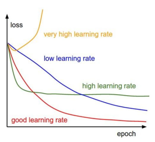
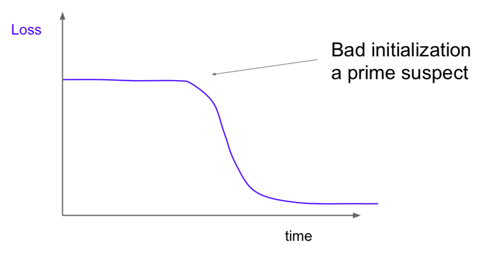
- start with small regularization and find learning rate that makes the loss go down
- loss barely changing = learning rate is too low
- cost: NaN = learning rate is too high
Hyperparameter Optimization
- cross-validation strategy
- coarse -> fine
- (tip) cost > 3 * original cost: break
- (tip) optimize in log space -> \(10^{(range)}\) (e.g. \(10^{(-5, 5)}\))
- order
- select candidates having validation accuracy
- narrow the range of hyperparameters
- if a candidate that exists at the edge is found, modify the range of hyperparameters
- random search vs grid search
- grid search: Assuming that all features are of equal importance, it is difficult to find the optimum.
- random search: Assuming that features are all different in importance, it is more likely to find the optimum point by exploring various points.
- visualization
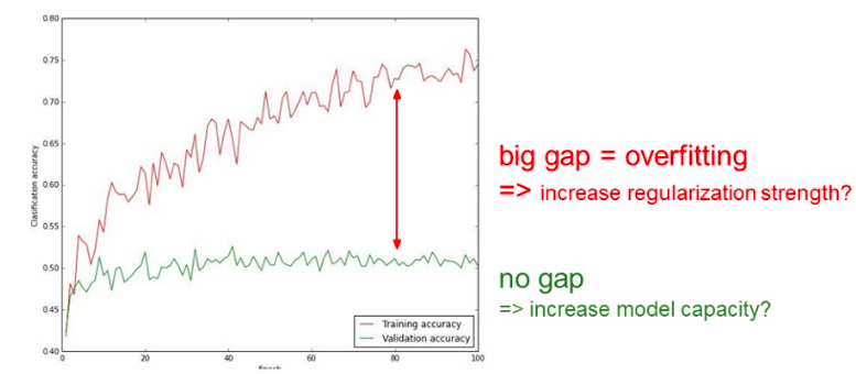
-
- big gap: can remove some features
-
- track the update ratio
- update scale / origin param scale
- want this to be somewhere around 0.001 or so
This is written by me after taking CS231n Spring 2017 provided by Stanford University.
If you have questions, you can leave a reply on this post.