Loss function
- \(x_i\): image, \(y_i\): label, \(L_i\): loss
- \[Loss = {1 \over N} \sum_i L_i(f(x_i, W), y_i) + Regulation\]
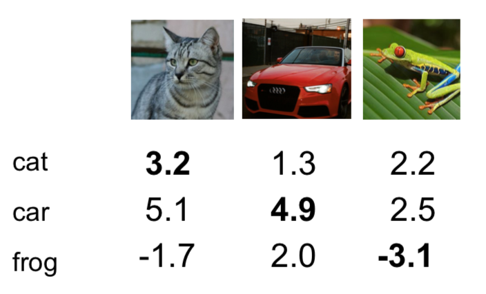
- Multiclass SVM loss
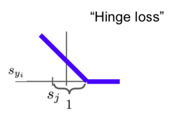
- \[L_i = \sum_{j \neq y_i} max(0, s_j - s_{y_i} + 1) \ (1: safety \ margin)\]
- Safety margin does not significantly affect the loss value result.
- \[L_{cat} = max(0, 5.1 - 3.2 + 1) + max(0, -1.7 -3.2 + 1) = 2.9\]
- \[L_{car} = max(0, 1.3 - 4.9 + 1) + max(0, 2.0 -4.9 + 1) = 0\]
- \[L_{frog} = max(0, 2.2 - (-3.1) + 1) + max(0, 2.5 - (-3.1) + 1) = 12.9\]
- \[L = (2.9 + 0 + 12.9) / 3 = 5.27\]
- Q. What happens to loss if car scores change a bit?
- A. No change -> since it is already higher than other scores, the loss continues to be zero
- Q. What is the min/max possible loss?
- A. min:0, max: \(\infty\)
- Q. At initialization W is small so all \(s \approx 0\). What is the loss?
- A. (number of class) - 1
- Q. What if the sum was over all classes? (including \(j = y_i\))
- A. the loss increases by 1
- Q. What if we used mean instead of sum?
- A. No change -> Only the scale of loss is different, but the same
- Q. What if we used \(L_i = \sum_{j \neq y_i} max (0, s_j - s_{y_i} + 1)^2\)
- A. loss increases -> different loss function
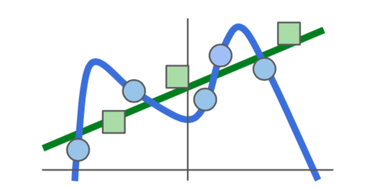
- Regularization
- because W, which makes loss zero, is not the only one, we adjust the loss value through regularization for test data.
- \[L(W) = {1 \over N} \sum_{i=1}^N L_i(f(x_i, W), y_i) + \lambda R(W) = Data \ loss + Regularization\]
- regularizations
- L1: makes feature with small weights converge to zero. In other words, it leaves only meaningful features.
- L2: decreases the overall weight of all features so that all features are considered. usually use this.
- Softmax Classifier
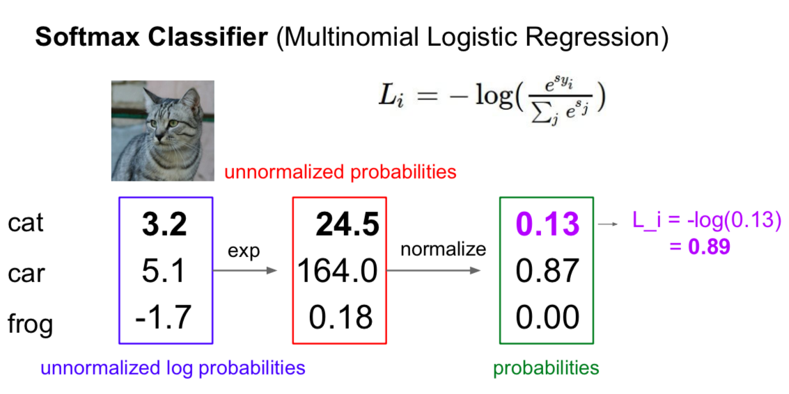
- Softmax function: \({e^{s_k} \over \sum_j e^{s_j}}\)
- \[L_i = -logP(Y = y_i | X = x_i) = -log({e^{s_k} \over \sum_j e^{s_j}})\]
- \[L_{cat} = 0.89\]
- Q. What is the min/max possibile loss \(L_i\)?
- A. min: 0, max: \(\infty\) (\(0 \leq probailities \leq 1\))
- Q. Usually at initialization W is small so all \(s \approx 0\). What is the loss?
- A. \(loss = {e^0 \over (e^0+e^0 + \cdots + e^0)} = log C\)
- Q. Suppose I take a datapoint and I jiggle a bit (changing its score slightly). What happens to the loss in Softmax and SVM cases
- SVM: No change
- Softmax: tries to make correct category to be infinity and incorrect categroy negative infinity, so the value continues to change.
Optimization
- Random search -> very bad idea
- Gradient descent
- 1-dimension: \({df(x) \ \over dx} = \lim_{h \rightarrow 0} {f(x+h) - f(x) \over h}\)
- multiple dimensions
- gradient: the vector of partial derivatives along each dimension
- slope: the dot product of the direction with the gradient
- Numerical gradient
- calculate one by one
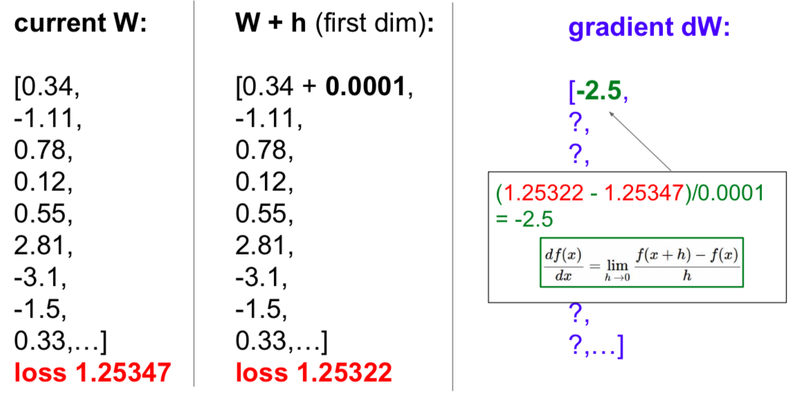
- approximate, slow, easy to write
- use it for debugging (= gradient check)
- Analytic gradient
- use calculus to compute
- exact, fast, error-prone
- use it in practice
- Gradient Descent
- weights += - step_size(= learning rate) * weights_gradient
- Stochastic Gradient Descent (SGD)
-
\[L(W) = {1 \over N} \sum_{i=1}^N L_i(x_i, y_i, W) + \lambda R(W)\]
- Full sum expensive when N is large = slow
-
\[\bigtriangledown_W L(W) = {1 \over N} \sum_{i=1}^N \bigtriangledown_W L_i(x_i, y_i, W) + \lambda \bigtriangledown_W R(W)\]
- Approximate sum using a minibatch of examples (32 / 64 /128 common)
-
\[L(W) = {1 \over N} \sum_{i=1}^N L_i(x_i, y_i, W) + \lambda R(W)\]
Image Features
- try
- use the image itself as a feature
- poor performance
- motivation
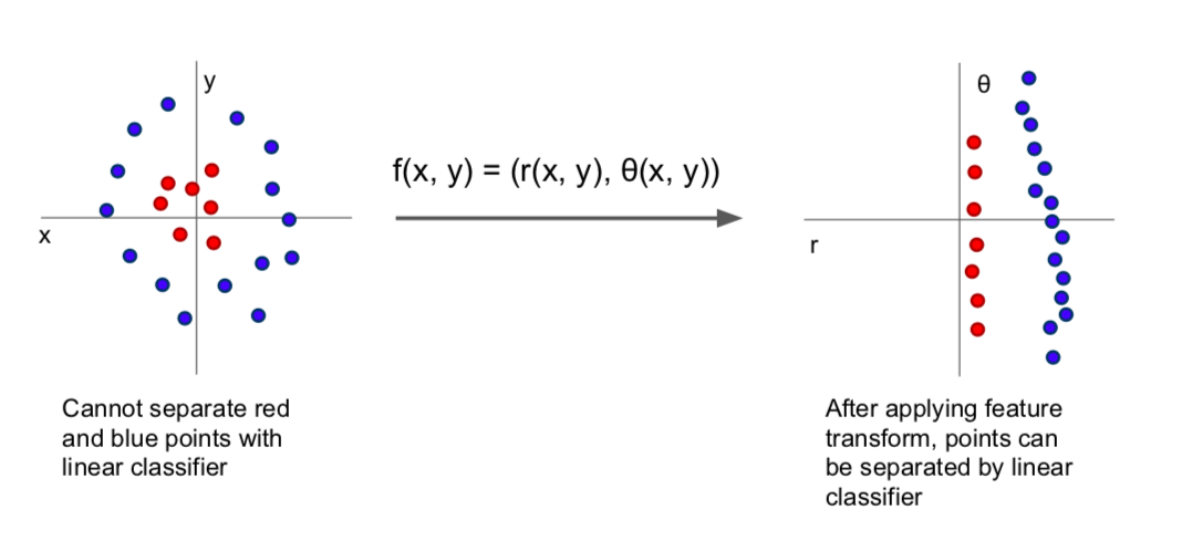
- points that could not be classified as linear classifiers have become possible in the polar coordinate system
- Color Histogram
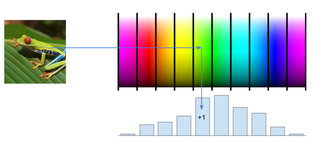
- extract the features of the image through the obtained hue values for every small part of the image
- Histogram of Oriented Gradients (HoG)
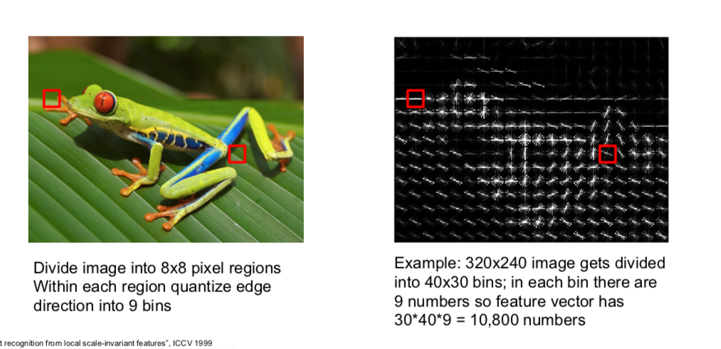
- when an image is cut into small pieces and the orientation value of that image is displayed as a histogram, the most orientation value is extracted as a feature
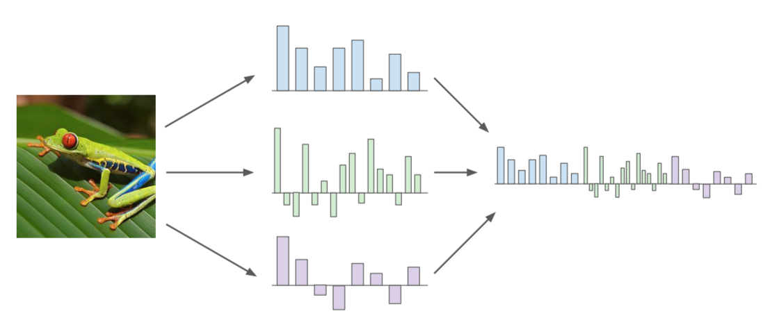
- Bag of Words
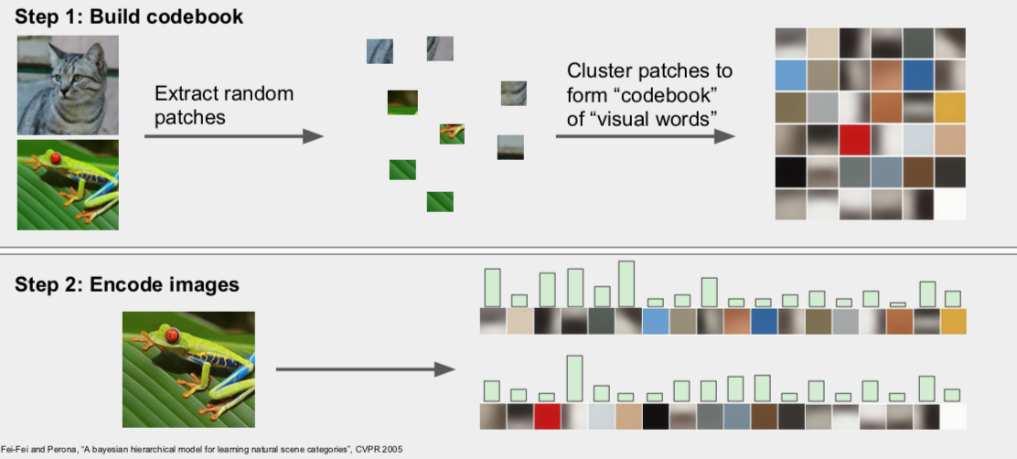
- the original image is divided into small pieces to form a cluster, and when a new image is introduced, it is cut and compared to the cluster’s features
- ConvNets
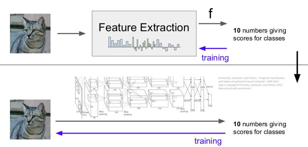
- during learning, features are extracted directly from the input image through filters, and these features are learned
This is written by me after taking CS231n Spring 2017 provided by Stanford University.
If you have questions, you can leave a reply on this post.