Previous Image Classification
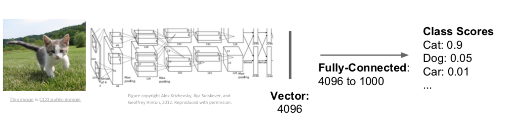
- images were classified through fully-connected layers of vectors obtained through neural network layers
Semantic Segmentation

- label each pixel in the image with a category label
- don’t differentiate instances, only care about pixels
- Idea: Sliding Window
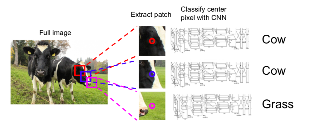
- split a image into small units and classify each part
- problems
- not reusing shared features between overlapping patches \(\rightarrow\) very inefficient
- check every pixel \(\rightarrow\) computationally expensive
- Idea: Fully Convolutional
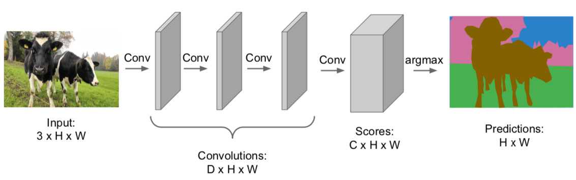
- C: number of categories
- design a network as a bunch of convolutional layers to make predictions for pixels all at once
- not use fully-connected layers
- for each pixel, the loss value is obtained and the average of the whole is used at training
- problems
- convolutions at original image resolution(no change in the spatial size) will be very expensive \(\rightarrow\) not use in practice
- Idea: Downsampling and Upsampling
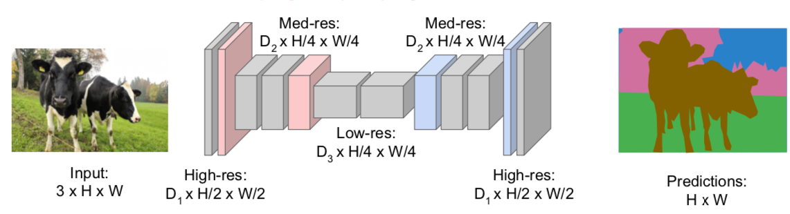
- design network as a bunch of convolutional layers, with downsampling and upsampling inside the network
- reduce the spatial size of the input and increase it again to equal the size of the input
- computationally efficient
- downsampling: pooling, strided convolution
- upsampling
- Unpooling
- Nearest Neighbor
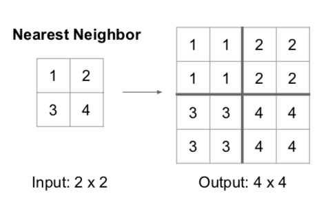
- fill in one part with the same number
- Bed of Nails
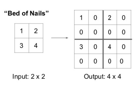
- each part will be filled with one input pixel and the rest will be filled with zero
- Nearest Neighbor
- Max Unpooling
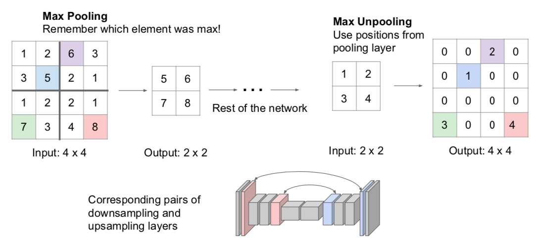
- remember locations of max values when Max Pooling, insert input pixel values at the positions when Max Unpooling, and fill the rest with zero
- remembering the location of the max values during Max Pooling does not require that much memory
- Transpose Convolution (Learnable Upsampling)
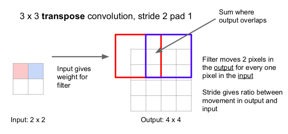
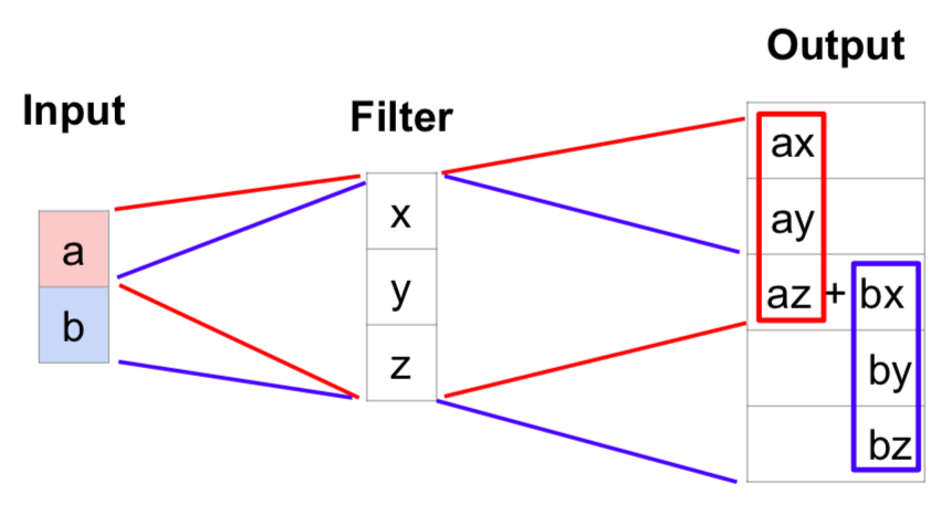
- the area is expanded through the calculation of the value(scala) of one area of input and the filter
- add the overlapping parts
- other names
- Deconvolution (not proper)
- Upconvolution
- Fractionally strided convolution
- Backward strided convolution
- Unpooling
Classification + Localization
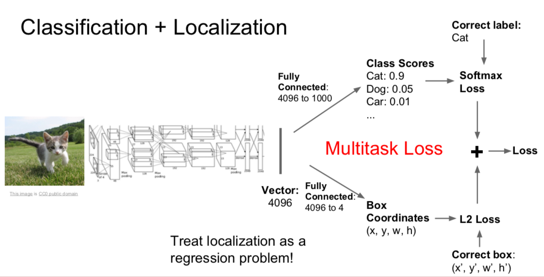
- find only one object and mark its location
- the final loss value is obtained by adding each of the two loss values
- when two loss values are added, the ratio is controlled by a hyperparameter
- two loss values can be backpropagated separately, but the performance is usually better when the two are combined and backpropagated as one value
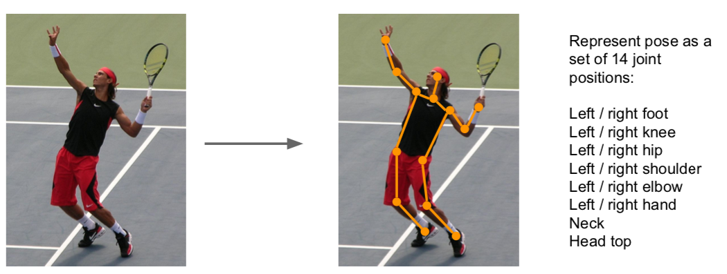
- Applied: Human Pose Estimation
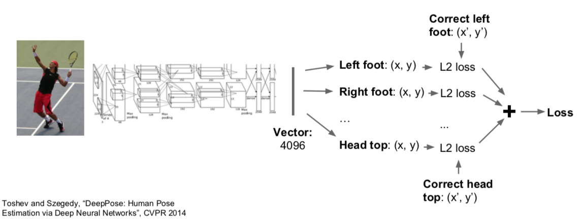
- when calculating loss, use regression loss
- the regression loss refers to calculating loss of continuous values rather than categorical values
Object Detection
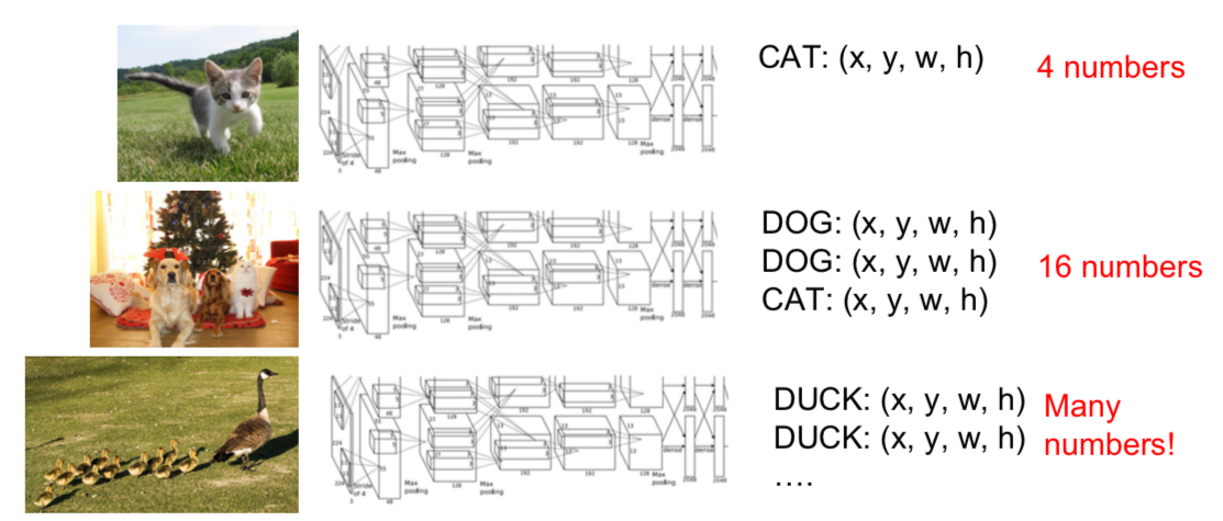
- Object Detection cannot use the same method as localization because it does not know how many objects to find
- Idea: Sliding Window
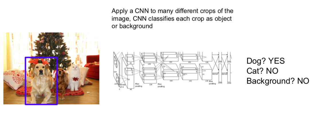
- need to apply CNN to huge number of locations and scales, very computationally expensive \(\rightarrow\) not use in practice
- Idea: Region Proposals
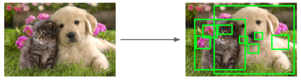
- not deep learning, but a traditional computer vision method
- find image regions that are expected to have objects (blobby image regions)
- relatively fast to run
- many regions are meaningless, but recall is high
- e.g. Selective Search gives 2000 region proposals in a few seconds on CPU
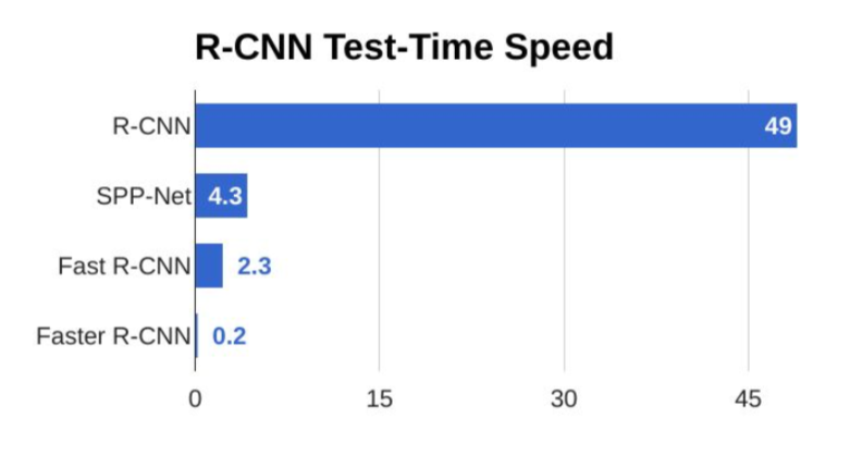
- Idea: R-CNN
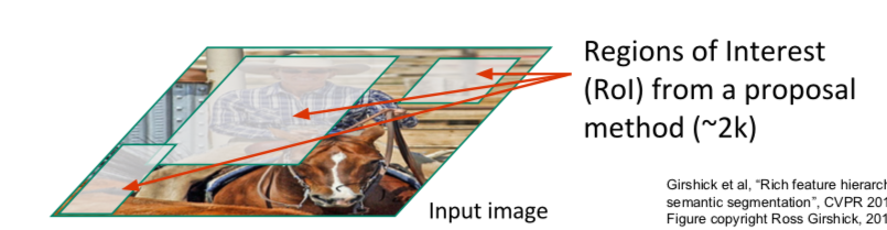
- find Region of Interest (= Region Proposals) when image input is received
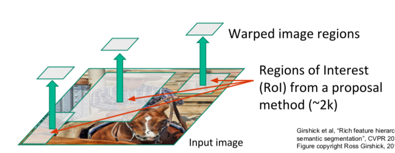
- since the size of the ROIs are all different, match them to the same size
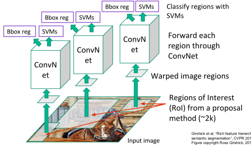
- problem
- training is slow (84h), takes a lot of disk space
- test time is also slow (30 sec)
- Idea: Fast R-CNN
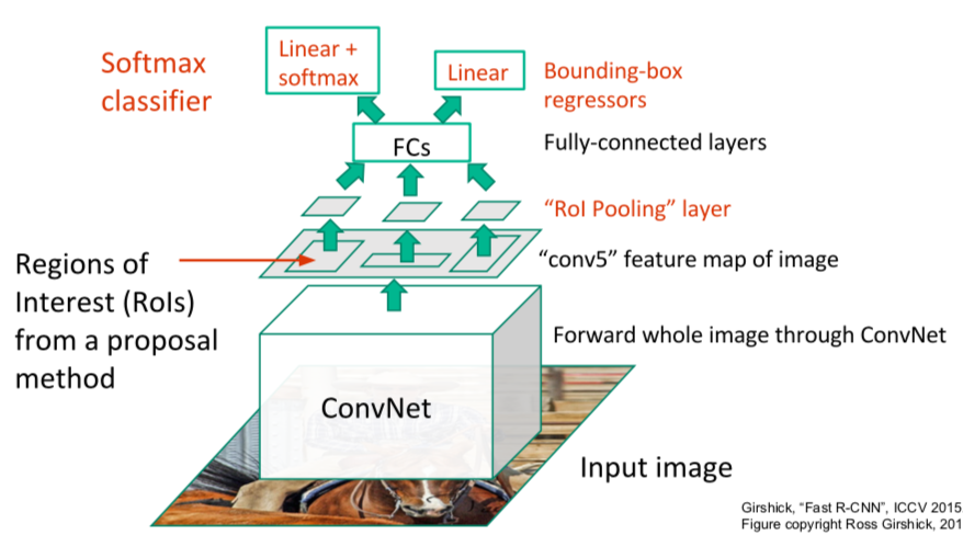
- ROI is not found for input image, and ROI is found in feature map after ConvNet
- it is performed outside the network when looking for ROI
- Make the size of the ROIs the same with the ROI Pooling Layer
- classification and regression are performed through a fully-connected layer
- final loss is a Multi-task loss obtained by adding two loss values and is used for backpropagation
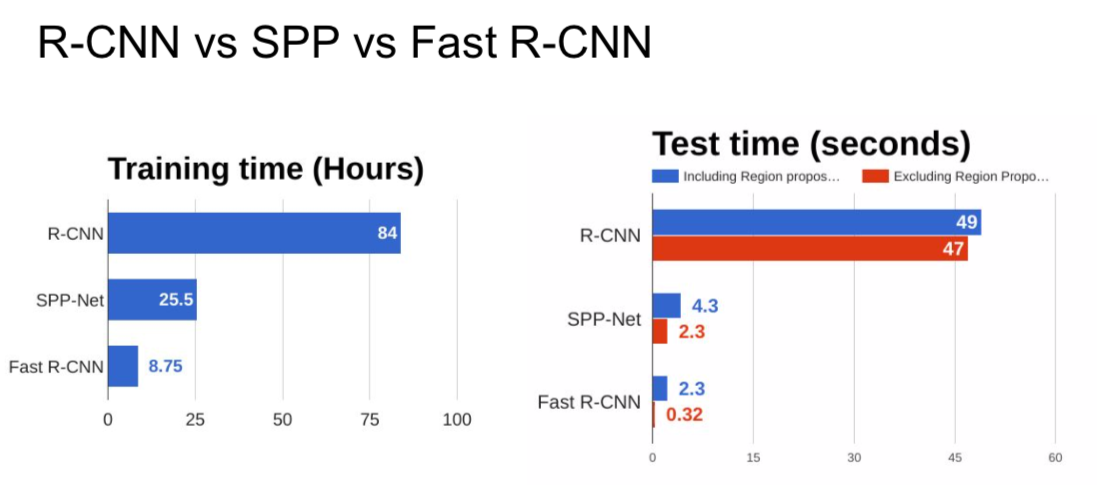
- problem: runtime dominated by region proposals
- Idea: Faster R-CNN
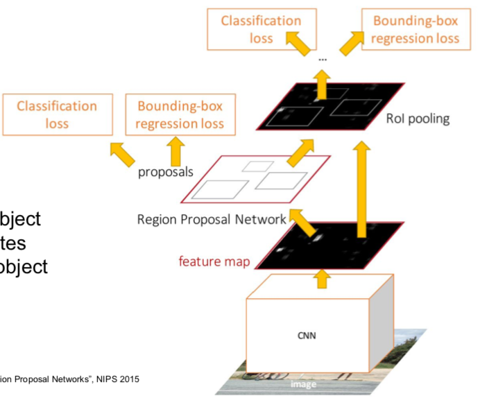
- when the input image comes in, a feature map is obtained through CNN
- Region Proposal is predicted in Region Proposal Network with feature map.
- after that, it goes through the same process as Fast R-CNN
- a total of four Loss values are calculated as shown in the figure
- Idea: YOLO / SSD
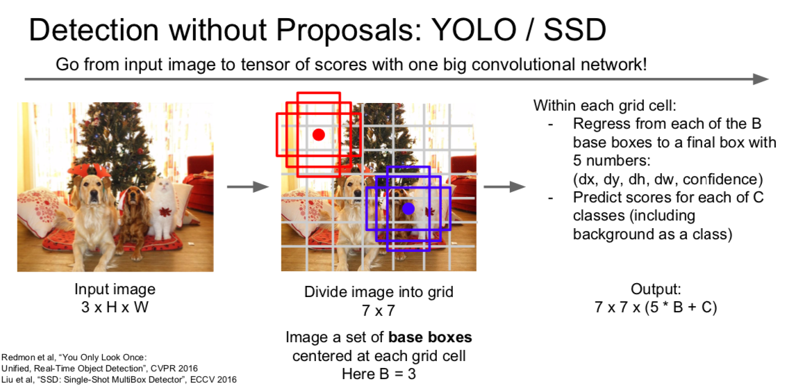
- when the image comes in, divide it into \(n \times n\) grid
- Bbase boxes are used for each grid cell (e.g., 3 but more in reality)
- Each grid cell is subjected to regression and classification to obtain \(n \times n \times (5 \times B + C)\) output
- dx, dy, dh, dw: offset between the actual object location and the Bbase box
- confidence: possibility that an object exists in the Bbase box
- Faster R-CNN is slower but more accurate
- SSD is much faster but not as accurate
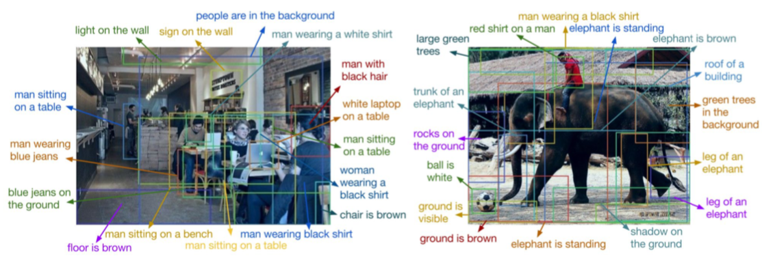
- Idea: Object Detection + Captioning = Dense Captioning
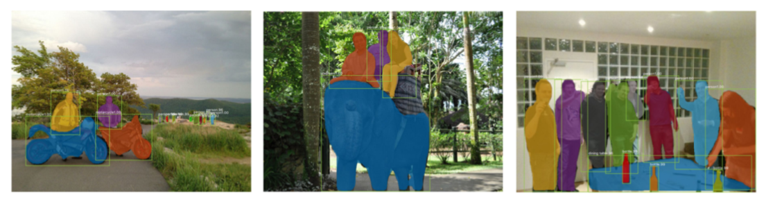
Instance Segmentation
- Semantic segmentation and object detection are mixed
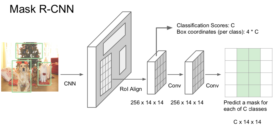
- find the ROI, classify the object, and find the bounding box
- in addition, through the same process as Semantic Segmentation, pixels belonging to the object are found
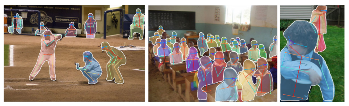
- possible if Joint Coordinates are found in the classification/regression process
This is written by me after taking CS231n Spring 2017 provided by Stanford University.
If you have questions, you can leave a reply on this post.