Visualize Filters
- First Layer
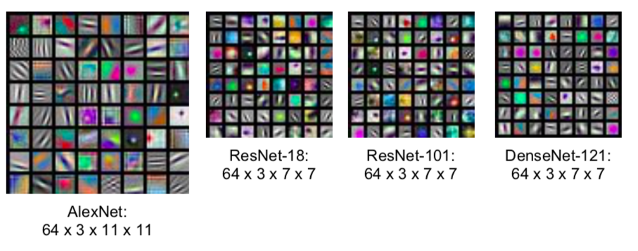
- a feature map created after passing through the first layer of ConvNet
- in the case of AlexNet, 64 3 x 11 x 11 feature maps are expressed in RGB
- feature map varies depending on the characteristics of the filter
- Middle Layers
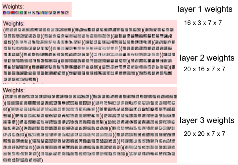
- visualize filters at higher layers, but not that interesting
- since it continues to be calculated on the feature map, the deeper it becomes, the more difficult it becomes to grasp the information
- Last Layer
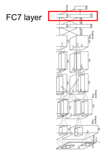
- layer immediately before the classifier
- since feature vectors are collected, meaningful information can be obtained
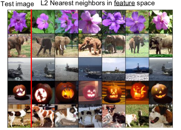
- Nearest neighbors were applied in pixel space
- In the case of elephant images, the test image has an elephant on the left, but the elephant image on the right is also classified as similar
- This is because it was judged that there was a similar feature in previous convolution layers
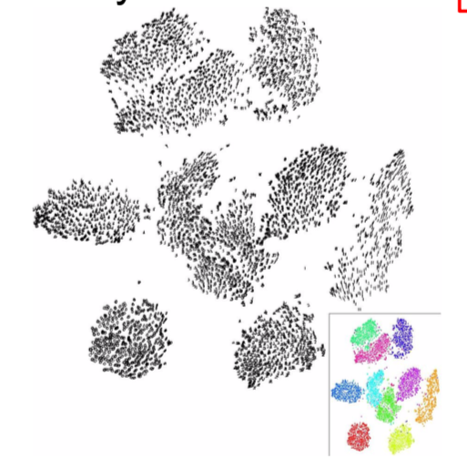
- The last layer also reduces the dimension
Visualizing Activations
- It was difficult to interpret when visualizing weights in the middle layer, but visualizing activation is sometimes interpretable.
- Maximally Activating Patches
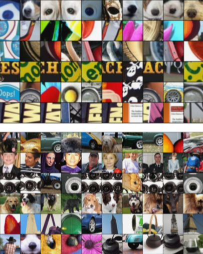
- One way to Visualize intermediate feature
- After training, select one layer and visualize image patches according to activation.
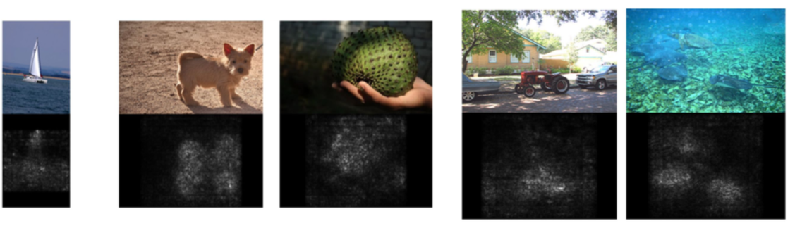
- Occlusion Experiments
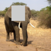
- A part of the image is occluded and the part is replaced with the average value of the image.
- When this image is put into the network, the change due to the occluded part is displayed as a heat map.
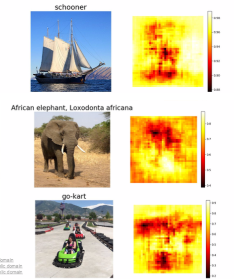
- The red part is the part where there is a significant change in the result when covered, and the yellow part has little effect.
- Therefore, it can be seen that the red area has a great influence on image classification.
- Saliency Maps
- Compute gradient of class score with respect to image pixels
- Simply put, for each pixel of the input image, check how much the class score changes when the pixel changes slightly
- We can see which pixels play an important role.
- Because the edges are well distinguished, it is also used for semantic segmentation
- Segmentation can be done without supervision, but the performance is very poor.
- Intermediate Features via (guided) backprop
- Pick a single intermediate neuron
- Compute gradient of neuron value with respect to image pixels
- Through this, it is possible to know which pixels affect the corresponding neuron.
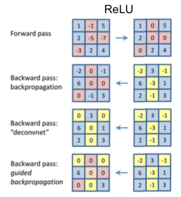
- Images come out nicer if you only backprop positive gradients through each ReLU (guided backprop)
- On the left side of the picture, there is a much clearer and better image through guided backprop.
- Visualized which pixels affect certain neurons.
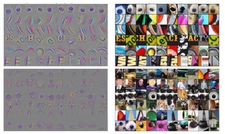
Visualizing CNN features: Gradient Ascent
- Through this, it is possible to answer which input generally activates neurons.
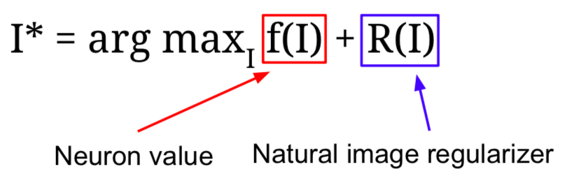
- I∗: Pixel value of the image
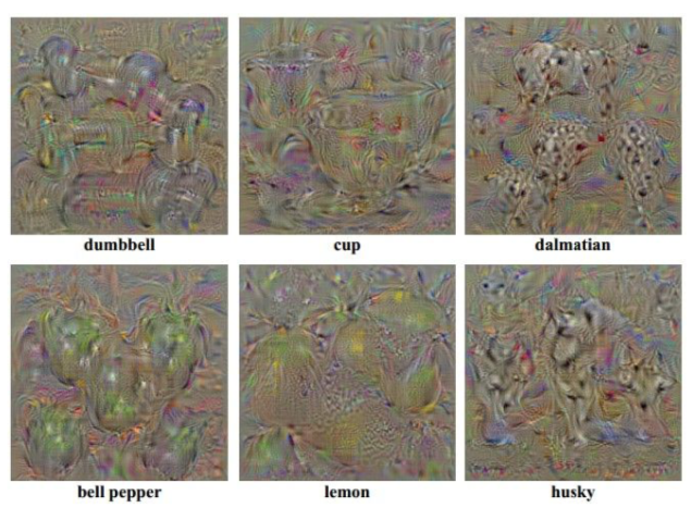
- It fixes all the weights of the network and generates pixels of images that maximize intermediate neurons or class scores through Gradient Ascent.
- Regularization term is used to prevent the generated image from being completely overfitted to the characteristics of a particular network when changing the pixel value of the input image so that the neuron, or class score can be maximized.
- How to carry it out
- Initialize image to zeros
- Forward image to compute current scores
- Backprop to get gradient of neuron value with respect to image pixels
- Make a small update to the image
- Repeat 2-4
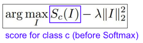
- L2 norm is used as regularization.
- Without regularization, the output would seem to be nothing.
- A better image can be created in the way presented in Jason Yesenski’s paper.
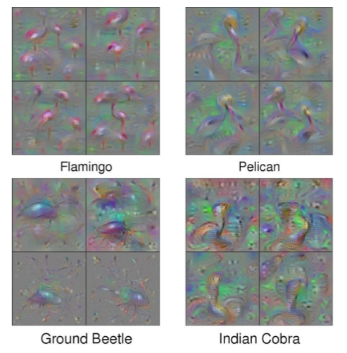
- during optimization periodically
- Gaussian blur image
- Clip pixels with small values to 0
- Clip pixels with small gradients to 0
- Adding “multi-faceted” visualization gives even nicer results: (Plus more careful regularization, center-bias)
Fooling Images / Adversarial Examples
- Start from an arbitrary image
- Pick an arbitrary class
- Modify the image to maximize the class
- Repeat until network is fooled
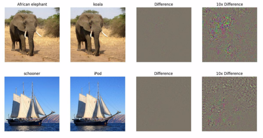
- In fact, even if the image is classified as the different label, there is no difference from the original picture.
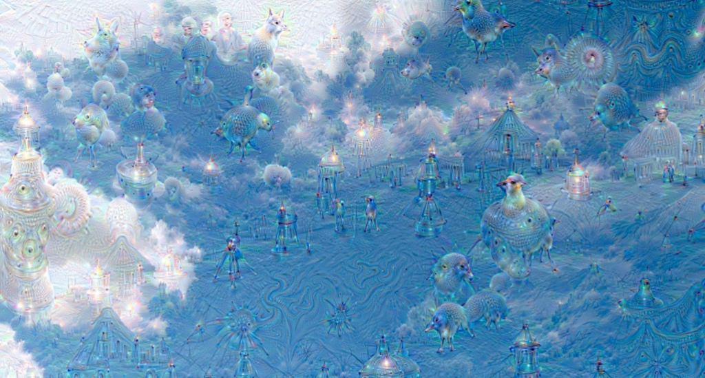
DeepDream: Amplify existing features
- It is to generate an funny image.
- Rather than synthesizing an image to maximize a specific neuron, instead try to amplify the neuron activations at some layer in the network
- Ways
- Forward: compute activations at chosen layer
- Set gradient of chosen layer equal to its activation (to amplify the features of the image)
- Backward: Compute gradient on image
- Update image
- Tricks
- Before calculating the gradients, jitters the image little bit
- It acts as a regularizer to generate a image that’s not awkward.
- L1 Normalization is also used (very useful in image synthesis)
- Clip the pixel value between 0 and 255.
Feature Inversion
- A way to guess what elements are being captured in various layers of the network.
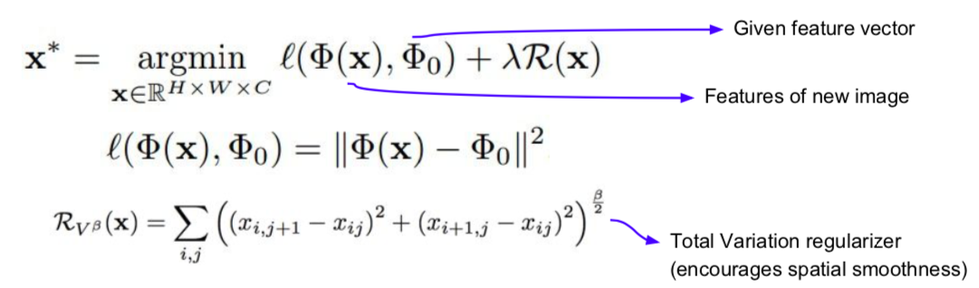
- Given a CNN feature vector for an image, find a new image that matches the given feature vector
- Generates an image that looks natural (way to minimize the distance between vectors)
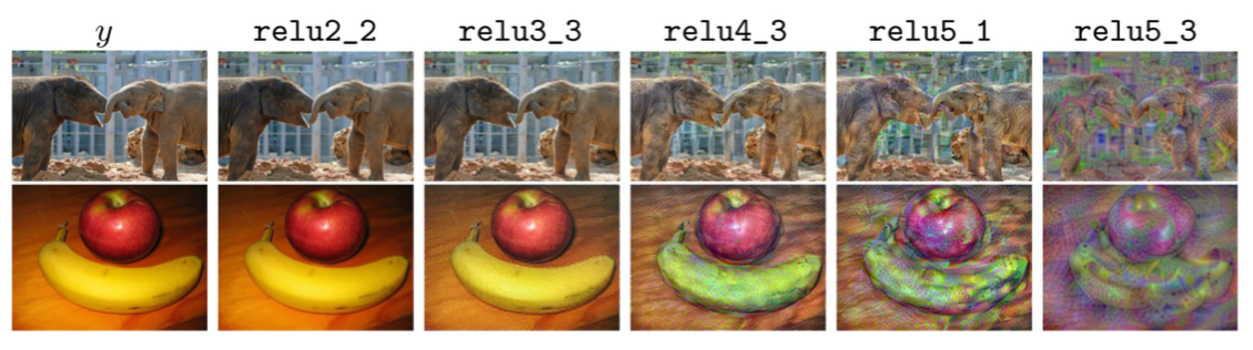
- Put images into the network to record a feature map, and generate new images that match the recorded feature map.
- Through images generated using various layers, it is possible to guess how much information is stored. (e.g., in the case of relu2_2, since it is almost similar to the original image, it can be seen that there is a lot of information.)
- As the network deepens, all of the low-level information, such as exactly how much the pixel value is, may disappear, and instead be trying to maintain only semantic information that is more robust to minor changes such as color and texture.
Texture Synthesis
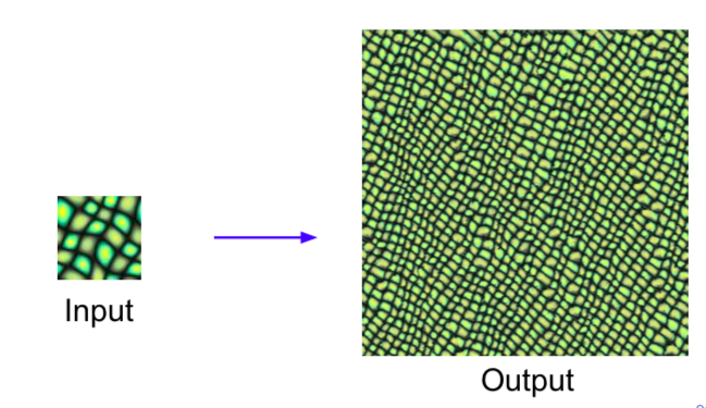
- Old: Nearest Neighbor
- Generate pixels one at a time in scanline order; form neighborhood of already generated pixels and copy nearest neighbor from input
- Doesn’t use neural networks.
- Doesn’t work well in the text.
- New: Gram Matrix
- Create a new matrix by out producting channels in different spatial information.
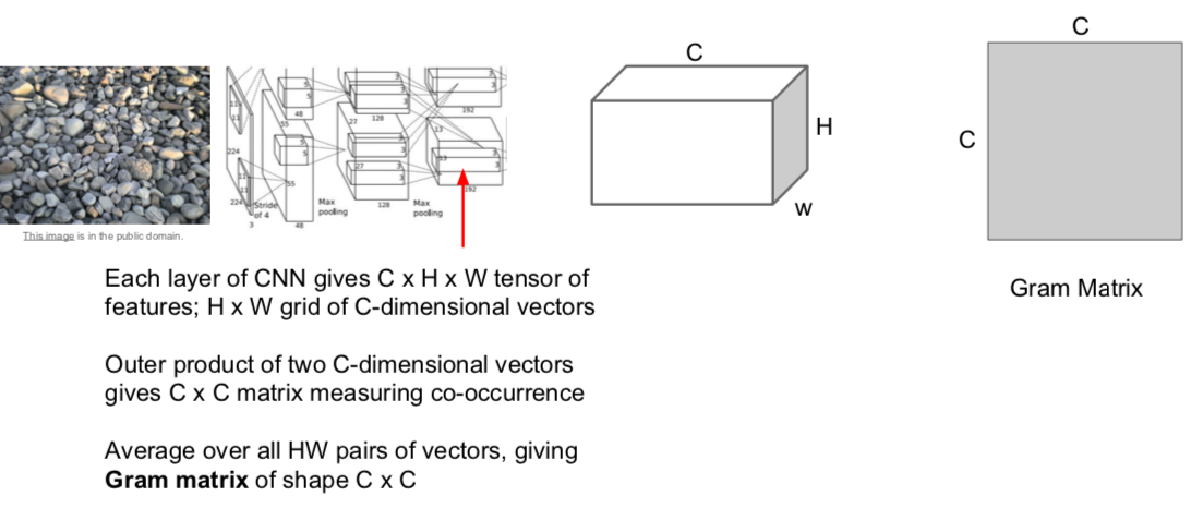
- The large value of the (i, j)th element of the CxC matrix means that both the i-th and j-th elements of the input vector are large.
- Through this, it is possible to capture to some extent through the secondary moment what features are activated in different spaces at the same time.
- Use the Gram matrix result as a texture descriptor describing the texture of the input image.
- Instead of averaging all the values corresponding to each point in the image and deleteing all spatial information, only co-occurrences between features are captured.
- Calculation is very efficient
- Way
- Pretrain a CNN on ImageNet (VGG-19)
- Run input texture forward through CNN, record activations on every layer; layer i gives feature map of shape \(C_i × H_i × W_i\)
- At each layer compute the Gram matrix giving outer product of features
- Initialize generated image from random noise
- Pass generated image through CNN, compute Gram matrix on each layer
- Compute loss: weighted sum of L2 distance between Gram matrices
- Backprop to get gradient on image
- Make gradient step on image
- GOTO 5
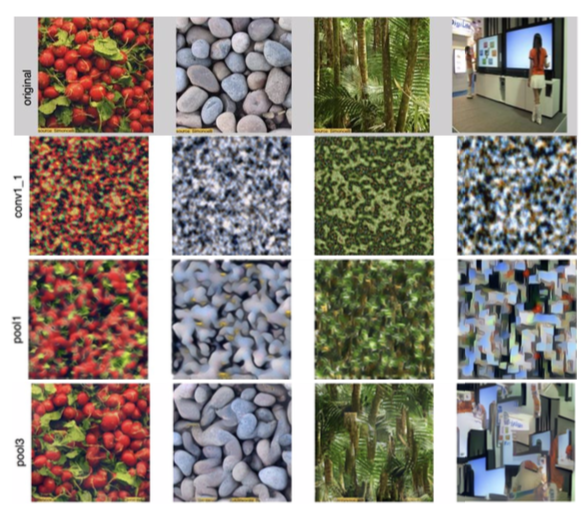
- Looking at the results in the shallow layer, the color is maintained well, but the spatial structure is not well utilized.
- The deeper the layer, the better it reconstructs the larger patterns of the image.
Neural Style Transfer
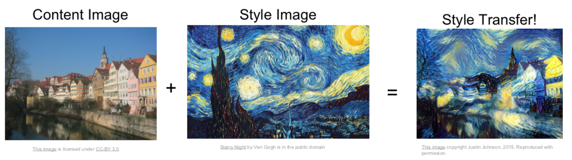
- Combination of texture synthesis and feature inversion
- Content Image: how you want our final image to be
- Style Image: what you want the texture to be like in the final image.
- The final image is generated by optimizing in a way that minimizes the feature reconstruction loss of the content image and minimizes the gram matrix loss of the style image.
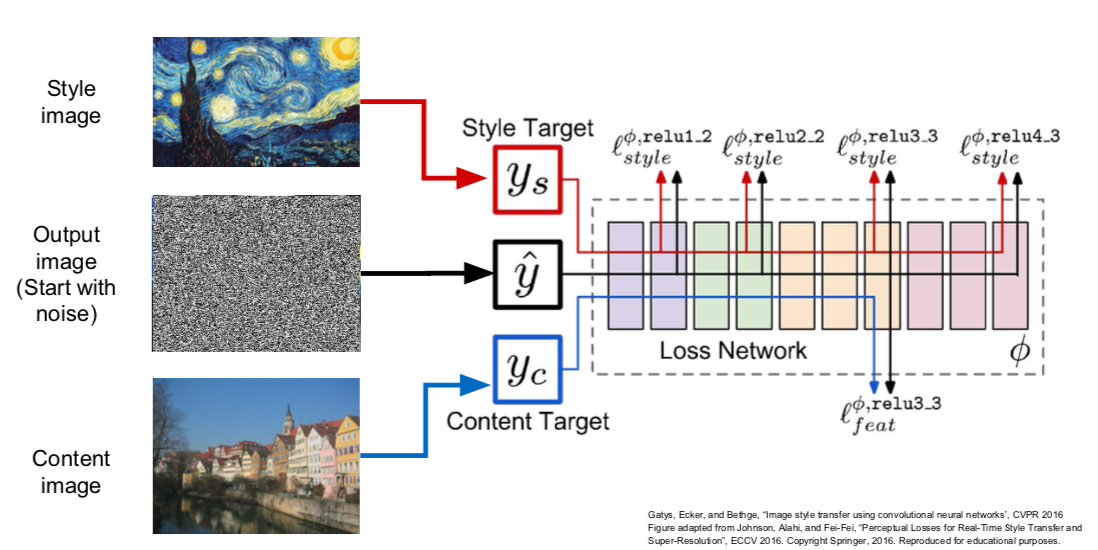
- Way
- Pass the content/style image through the network and calculate the gram matrix and feature map.
- The final output image is initialized to random noise.
- Repeat the forward/backward calculation and update the image using gradient ascent.
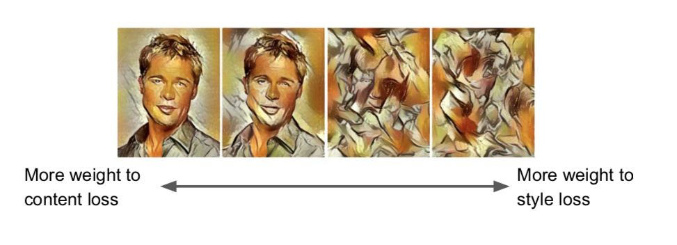
- Changes can be made through various parameter adjustments.
- Problem
- Style transfer requires many forward / backward passes through VGG; very slow!
- Solution: Train another neural network to perform style transfer for us
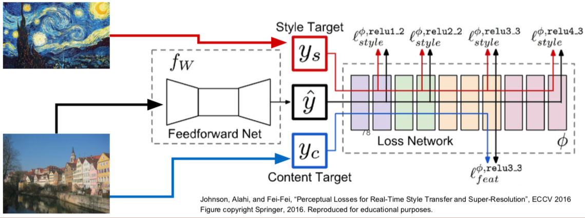
- Train a feedforward network for each style
- Use pretrained CNN to compute same losses as before
- After training, stylize images using a single forward pass
This is written by me after taking CS231n Spring 2017 provided by Stanford University.
If you have questions, you can leave a reply on this post.